Linear Dielectrics

Original learning note in English

Original Korean learning note, published November 19, 2014. The translation follows its full text and image order. The historical image links preserve the original notation; dated notes clarify mistakes, and the scientific appendix gives the complete corrected explanation.

Now let’s think a little more about this \(\mathbf P\) in \(\mathbf D=\varepsilon\mathbf E+\mathbf P\)!

Editorial note (2026-10-02): The opening source line uses \(\varepsilon\), but the SI definition is \(\mathbf D=\varepsilon_0\mathbf E+\mathbf P\). The later source derivation uses \(\varepsilon_0\) correctly. Here \(\varepsilon\) denotes the material permittivity.

Way back earlier, we introduced polarization through \(\mathbf p=\alpha\mathbf E\),

Editorial note (2026-10-02): For the microscopic relation, the field acting on an atom is the local field \(\mathbf E_{\mathrm{local}}\). It need not equal the macroscopic field in the constitutive relation.

and called alpha the atomic polarizability: a measure of how that atom responds to an electric field.

So it seems each atom should have its own characteristic value of alpha.

A large alpha means a larger \(\mathbf p\) than in another material for the same \(\mathbf E\): more polarization, or easier polarization. A small alpha would mean the opposite.

That was for an atom. For an entire object, it is almost impossible to consider atoms one by one, so we introduced \(\mathbf P\) instead of \(\mathbf p\).

Since \(\mathbf P\) means dipole moment \(\mathbf p\) per unit volume, it should also be proportional to the electric field, just like \(\mathbf p\).

Hmm~ well, about that…..

It is proportional in the case of a linear dielectric.

We will consider these linear dielectrics.

In other words, we will deal with the case where polarization is proportional to the electric field.

For a linear dielectric,

Historical source image 1: Polarization equals vacuum permittivity times electric susceptibility times the total electric field.

\[ \mathbf P=\varepsilon_0\chi_e\mathbf E. \]

this relation holds. If this equation holds, we have a linear dielectric~

Editorial note (2026-10-02): The scalar form displayed here assumes an isotropic linear dielectric. In an anisotropic linear dielectric, electric susceptibility is generally a tensor.

(We pulled out epsilon zero to make chi a dimensionless number. Now chi depends on the material’s structure… it is like alpha from earlier!!)

Anyway, chi is a proportionality constant determined by conditions such as the structure or temperature of the material.

It is called electric susceptibility in English; the Korean term means the same thing.

Oh, and \(\mathbf E\) above is the total electric field.

That \(\mathbf E\) includes all kinds of electric fields apart from the polarization contribution, plus the effect due to polarization: everything is counted.

Now, if an object is placed in an electric field \(\mathbf E_0\), we cannot obtain the total field \(\mathbf E\) from \(\mathbf E_0\) and \(\mathbf P\)…

Editorial note (2026-10-02): This is a difficulty of self-consistency, rather than an impossibility theorem. If the full polarization distribution and geometry are known, its bound charges determine its field. To find an initially unknown polarization, solve the electrostatic boundary problem together with \(\mathbf P=\varepsilon_0\chi_e\mathbf E\). The repeated sentence below is retained from the original.

Now, if an object is placed in the electric field \(\mathbf E_0\),

we cannot obtain the total field \(\mathbf E\) using \(\mathbf E_0\) and \(\mathbf P\).

Because \(\mathbf E_0\) produces \(\mathbf P\), then \(\mathbf P\) produces another \(\mathbf E\), and that other \(\mathbf E\) changes \(\mathbf P\) to make a new \(\mathbf P\), and so on…

This process goes on forever…….. sigh~~~~

That is why we learned about the displacement field earlier!!! The field due to \(\rho_{\mathrm{free}}\)!!!

Editorial note (2026-10-02): The displacement field is an auxiliary field with \(\nabla\cdot\mathbf D=\rho_f\); it is not the physical electric field produced only by free charge. Its flux is fixed by enclosed free charge, and geometry and constitutive relations are still needed.

So,

Historical source image 2: Substitution into the displacement-field definition; call epsilon zero times one plus chi e epsilon, and therefore D equals epsilon E.

\[ \begin{aligned} \mathbf D&=\varepsilon_0\mathbf E+\mathbf P=\varepsilon_0\mathbf E+\varepsilon_0\chi_e\mathbf E\\ &=\varepsilon_0(1+\chi_e)\mathbf E.\\ \varepsilon_0(1+\chi_e)&=\varepsilon\quad\text{(let us call this epsilon)}.\\ \therefore\quad\mathbf D&=\varepsilon\mathbf E. \end{aligned} \]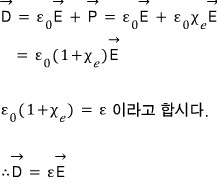

this lets us derive a relation.

Here, epsilon is called permittivity.

With chi (electric susceptibility) and epsilon (permittivity) suddenly appearing, it is pretty confusing, right?

Let’s go over the roles of those constants!!!!

First, chi (electric susceptibility) is related to polarization.

It is similar to the atomic polarizability alpha we used earlier when looking at atoms microscopically:

a large chi for a dielectric means it polarizes readily, and the opposite case means the opposite.

Okay, okay, once again: chi tells us how readily (or how much) polarization occurs.

Now let’s look at permittivity. It appears in the relation between the displacement field and the total electric field.

First, a larger chi means stronger polarization, right???

What happens when polarization is stronger? It cancels some of the external electric field, right??? ((Because it creates a new electric field opposite to the direction of \(\mathbf P\).))

Then the total electric field will be somewhat smaller than the external field.

Editorial note (2026-10-02): This reduction is valid for the ordinary electrostatic dielectric configuration being discussed, with a depolarizing field. A polarization field is not universally opposite to \(\mathbf P\) at every point or in every geometry. For the fixed-free-charge spherical shell below, \(\mathbf E=\mathbf D/\varepsilon\) makes the reduction precise.

Aha!

A large chi means a large epsilon, and a large epsilon means greater cancellation of the external electric field.

A small chi means a small epsilon, and a small epsilon means less cancellation of the external electric field.

Let’s solve a problem.

Historical source image 4: A charge Q has been placed in a metal sphere of radius a. A linear dielectric of permittivity epsilon, with outer radius b, surrounds it. Find the potential at the center.

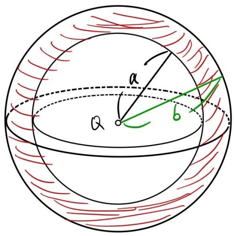
It is asking for the potential \(V\). How should we find \(V\)?

We could add all the potentials produced by the surface or volume charge densities at each point, but the integral would become too complicated….

Besides, this problem involves a sphere, so there is symmetry.

Aha, how about finding the electric field with Gauss’s law and then integrating the electric field???

Since there is a dielectric, let’s use the displacement vector \(\mathbf D\) to find the total electric field \(\mathbf E\), and then find \(V\), rather than trying to find \(\mathbf E\) directly.

Since it is a conducting sphere, for \(r\lt a\) we have \(Q_{\mathrm{in}}=0\), so the total electric field is zero without even having to look further.

Editorial note (2026-10-02): Zero field inside the metal follows from electrostatic equilibrium. Zero enclosed charge alone does not prove zero field in an arbitrary geometry; the spherical symmetry here also makes the Gaussian argument valid.

Then we will examine just two cases.

Historical source image 5: First case, inside the dielectric shell, a less than r less than b; Gaussian flux gives D and then E.

\[ \begin{aligned} \text{i)}\quad&a\lt r\lt b,\\ D(4\pi r^2)&=Q_{\mathrm{in(free)}}=Q,\\ \therefore\quad\mathbf D&=\frac{Q}{4\pi r^2}\hat{\mathbf r}=\varepsilon\mathbf E,\\ \therefore\quad\mathbf E&=\frac{1}{4\pi\varepsilon}\frac{Q}{r^2}\hat{\mathbf r}. \end{aligned} \]

Historical source image 6: Second case, outside the dielectric shell, r greater than b; polarization is zero and the vacuum electric field follows.

\[ \begin{aligned} \text{ii)}\quad&r\gt b,\\ D(4\pi r^2)&=Q_{\mathrm{in(free)}}=Q,\\ \therefore\quad\mathbf D&=\frac{Q}{4\pi r^2}\hat{\mathbf r}=\varepsilon_0\mathbf E+\mathbf P\;(=0),\\ \therefore\quad\mathbf E&=\frac{1}{4\pi\varepsilon_0}\frac{Q}{r^2}\hat{\mathbf r}. \end{aligned} \]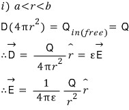

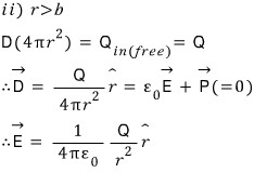
Editorial note (2026-10-02): The source notation \(\mathbf P\;(=0)\) means polarization is zero in the exterior vacuum; it does not mean \(\mathbf D\) or \(\mathbf E\) is zero.

Now let’s integrate over the intervals.

Historical source image 7: Potential at the center from three radial integration intervals: infinity to b, b to a, and a to zero.

\[ \begin{aligned} V&=-\int_\infty^0\mathbf E\,d\hat{\mathbf r}\\ &=-\left\{\int_\infty^b\frac{1}{4\pi\varepsilon_0}\frac{Q}{r^2}\hat{\mathbf r}\,d\hat{\mathbf r} +\int_b^a\frac{1}{4\pi\varepsilon}\frac{Q}{r^2}\hat{\mathbf r}\,d\hat{\mathbf r} +\int_a^0 0\,d\hat{\mathbf r}\right\}\\ &=\left\{\frac{1}{4\pi\varepsilon_0}\frac{Q}{b}+\frac{1}{4\pi\varepsilon}Q\left(\frac1a-\frac1b\right)\right\}\\ &=\frac{Q}{4\pi}\left\{\frac{1}{\varepsilon_0b}+\frac{1}{\varepsilon a}-\frac{1}{\varepsilon b}\right\}. \end{aligned} \]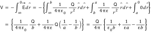

Editorial note (2026-10-02): The source writes the differential as \(d\hat{\mathbf r}\), without a dot product. This is retained above only as historical notation. The correct potential integral is \(V(0)=-\int_\infty^0\mathbf E\cdot d\boldsymbol\ell=-\int_\infty^0 E_r\,dr\), with \(V(\infty)=0\). The final scalar expression is correct for the potential throughout the conductor.

And one more thing!!! Since we know the total field \(\mathbf E\) in the dielectric region, we can also find the bound charge densities!

Historical source image 8: Polarization, zero bound volume charge, and bound surface charge on the inner and outer dielectric interfaces.

\[ \begin{aligned} \mathbf P(r)&=\varepsilon_0\chi_e\mathbf E(r)=\varepsilon_0\chi_e\frac{1}{4\pi\varepsilon}\frac{Q}{r^2}\hat{\mathbf r},\\ \therefore\quad\rho_b&=-\nabla\cdot\mathbf P(r) =-\frac{1}{r^2}\frac{\partial}{\partial r}r^2\left(\varepsilon_0\chi_e\frac{1}{4\pi\varepsilon}\frac{Q}{r^2}\right)=0,\\ \therefore\quad\sigma_{b(\mathrm{inner})}&=\mathbf P(a)\cdot(-\hat{\mathbf r}) =-\varepsilon_0\chi_e\frac{1}{4\pi\varepsilon}\frac{Q}{a^2},\\ \therefore\quad\sigma_{b(\mathrm{outer})}&=\mathbf P(b)\cdot(\hat{\mathbf r}) =\varepsilon_0\chi_e\frac{1}{4\pi\varepsilon}\frac{Q}{b^2}. \end{aligned} \]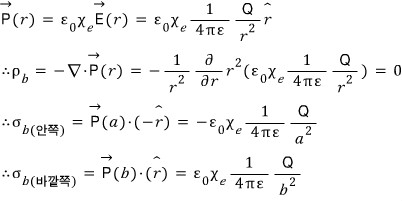

Editorial note (2026-10-02): The zero volume density applies in the open homogeneous shell \(a\lt r\lt b\). The two interface charges remain: the outward normal of the dielectric is inward at its inner boundary and outward at its outer boundary.

Scientific appendix: the complete corrected explanation

We introduced the dipole moment of an atom or molecule through a relation such as

\[ \mathbf p=\alpha\mathbf E_{\mathrm{local}}, \]

where \(\alpha\) is the atomic or molecular polarizability. A larger \(\alpha\) means that the same local electric field induces a larger dipole moment.

For a macroscopic material, tracking every microscopic dipole is impractical. Instead we use the polarization \(\mathbf P\), the electric dipole moment per unit volume. In a simple isotropic linear dielectric, the macroscopic constitutive relation is

\[ \boxed{\mathbf P=\varepsilon_0\chi_e\mathbf E}, \]

where \(\chi_e\) is the dimensionless electric susceptibility and \(\mathbf E\) is the total macroscopic electric field in the material. The factor \(\varepsilon_0\) is included so that \(\chi_e\) has no units.

This scalar relation assumes a linear, isotropic medium. If the material is anisotropic, susceptibility is generally a tensor; if its response is nonlinear, \(\mathbf P\) is not simply proportional to \(\mathbf E\). Both \(\chi_e\) and the resulting permittivity can also depend on temperature and, for time-dependent fields, frequency.

Susceptibility, permittivity, and the displacement field

The electric displacement field is defined by

\[ \mathbf D=\varepsilon_0\mathbf E+\mathbf P. \]

Substituting the linear constitutive relation gives

\[ \mathbf D =\varepsilon_0\mathbf E+\varepsilon_0\chi_e\mathbf E =\varepsilon_0(1+\chi_e)\mathbf E =\varepsilon\mathbf E, \]

with

\[ \boxed{\varepsilon=\varepsilon_0(1+\chi_e)}. \]

So \(\chi_e\) measures how strongly the material polarizes, while \(\varepsilon\) connects \(\mathbf D\) to the total macroscopic field \(\mathbf E\) in this isotropic linear medium.

In electrostatics,

\[ \nabla\cdot\mathbf D=\rho_f, \qquad \oint_S\mathbf D\cdot d\mathbf a=Q_{f,\mathrm{enc}}. \]

This is why \(\mathbf D\) is so useful: its flux is determined by free charge, while polarization is absorbed into the constitutive relation. But \(\mathbf D\) should not be described as “the electric field produced by free charge.” It is an auxiliary field, and the physical electric field is still \(\mathbf E\).

For a fixed free-charge distribution in a simple geometry, a larger \(\varepsilon\) produces a smaller \(\lvert\mathbf E\rvert=\lvert\mathbf D\rvert/\varepsilon\) inside the dielectric. That reduction is the macroscopic effect of the bound charges created by polarization.

Example: conducting sphere with a dielectric shell

Diagram already shown above: A conducting sphere of radius a surrounded by a concentric dielectric shell extending to radius b

A conducting sphere of radius \(a\) carries total free charge \(Q\). A homogeneous, isotropic, linear dielectric of permittivity \(\varepsilon\) fills the concentric shell from \(r=a\) to \(r=b\). The region outside the shell is vacuum. Find \(\mathbf D\), \(\mathbf E\), the potential \(V\), and the bound charges.

We assume electrostatic equilibrium, spherical symmetry, and \(V(\infty)=0\). The free charge lies on the conductor surface. There is no additional free charge in the dielectric or at its outer boundary.

Displacement field

Inside the conductor, the electrostatic field vanishes. For a spherical Gaussian surface with \(r\gt a\), the enclosed free charge is \(Q\), so

\[ 4\pi r^2D_r=Q. \]

Therefore

\[ \boxed{ \mathbf D(r)= \begin{cases} \mathbf 0, & 0\le r\lt a,\\[4pt] \displaystyle\frac{Q}{4\pi r^2}\,\hat{\mathbf r}, & r\gt a. \end{cases}} \]

At \(r=a\), the normal component jumps by the free surface-charge density

\[ \sigma_f=\frac{Q}{4\pi a^2}. \]

At \(r=b\), there is no free surface charge, so the normal component of \(\mathbf D\) is continuous.

Electric field

Use \(\mathbf D=\varepsilon\mathbf E\) in the dielectric and \(\mathbf D=\varepsilon_0\mathbf E\) in vacuum:

\[ \boxed{ \mathbf E(r)= \begin{cases} \mathbf 0, & 0\le r\lt a,\\[4pt] \displaystyle\frac{Q}{4\pi\varepsilon r^2}\,\hat{\mathbf r}, & a\lt r\lt b,\\[8pt] \displaystyle\frac{Q}{4\pi\varepsilon_0 r^2}\,\hat{\mathbf r}, & r\gt b. \end{cases}} \]

The field is smaller in the dielectric than it would be in vacuum by the factor \(\varepsilon_0/\varepsilon\).

Potential

For \(r\gt b\), integration from infinity gives

\[ V(r)=\frac{Q}{4\pi\varepsilon_0r}. \]

For \(a\lt r\lt b\), split the integral at the material boundary:

\[ \begin{aligned} V(r) &=\int_r^b\frac{Q}{4\pi\varepsilon r'^2}\,dr' +\int_b^\infty\frac{Q}{4\pi\varepsilon_0 r'^2}\,dr'\\[4pt] &=\frac{Q}{4\pi} \left[ \frac{1}{\varepsilon}\left(\frac{1}{r}-\frac{1}{b}\right) +\frac{1}{\varepsilon_0b} \right]. \end{aligned} \]

The conductor is an equipotential, so for \(0\le r\le a\),

\[ V(r)=V(a)=\frac{Q}{4\pi} \left[ \frac{1}{\varepsilon}\left(\frac{1}{a}-\frac{1}{b}\right) +\frac{1}{\varepsilon_0b} \right]. \]

Collecting the three regions,

\[ \boxed{ V(r)= \begin{cases} \displaystyle\frac{Q}{4\pi} \left[ \frac{1}{\varepsilon}\left(\frac{1}{a}-\frac{1}{b}\right) +\frac{1}{\varepsilon_0b} \right], & 0\le r\le a,\\[12pt] \displaystyle\frac{Q}{4\pi} \left[ \frac{1}{\varepsilon}\left(\frac{1}{r}-\frac{1}{b}\right) +\frac{1}{\varepsilon_0b} \right], & a\lt r\lt b,\\[12pt] \displaystyle\frac{Q}{4\pi\varepsilon_0r}, & r\gt b. \end{cases}} \]

Both \(V\) and the tangential component of \(\mathbf E\) are continuous at each interface. The normal component of \(\mathbf E\) changes at \(r=b\) because the permittivity changes.

The capacitance of this isolated, dielectric-coated sphere relative to infinity follows from \(C=Q/V(a)\):

\[ \boxed{ C=\frac{4\pi}{ \displaystyle \frac{1}{\varepsilon}\left(\frac{1}{a}-\frac{1}{b}\right) +\frac{1}{\varepsilon_0b}} }. \]

Polarization and bound charge

Within the dielectric shell,

\[ \begin{aligned} \mathbf P &=(\varepsilon-\varepsilon_0)\mathbf E\\[3pt] &=\left(1-\frac{\varepsilon_0}{\varepsilon}\right) \frac{Q}{4\pi r^2}\,\hat{\mathbf r}, \qquad a\lt r\lt b. \end{aligned} \]

Because \(r^2P_r\) is constant in the homogeneous shell,

\[ \boxed{\rho_b=-\nabla\cdot\mathbf P=0} \qquad(a\lt r\lt b). \]

The bound surface-charge density is \(\sigma_b=\mathbf P\cdot\hat{\mathbf n}\), where \(\hat{\mathbf n}\) points outward from the dielectric. At the inner surface that outward normal is \(-\hat{\mathbf r}\); at the outer surface it is \(+\hat{\mathbf r}\). Hence

\[ \boxed{ \sigma_b(a)=-\left(1-\frac{\varepsilon_0}{\varepsilon}\right) \frac{Q}{4\pi a^2}} \]

and

\[ \boxed{ \sigma_b(b)=+\left(1-\frac{\varepsilon_0}{\varepsilon}\right) \frac{Q}{4\pi b^2}}. \]

The total bound charge on the two interfaces is

\[ 4\pi a^2\sigma_b(a)+4\pi b^2\sigma_b(b)=0, \]

as expected for a neutral dielectric whose polarization merely separates charge. The negative bound charge on the inner surface partially screens the conductor’s positive free charge within the dielectric, while the positive bound charge on the outer surface restores the full vacuum field outside.