The Method of Images: A Charge Above a Grounded Plane

Original study note — faithful English narrative

Read the reviewed scientific explanation.

Source narrative restored (2 October 2026). The following translation preserves the explanations, jokes, and historical claims in the original note of 16 November 2014. Some historical claims are incorrect or incomplete. The three affected historical images are linked as source references, and the complete previously reviewed scientific derivation follows this narrative. Use that derivation for the corrected field, conductor boundary, surface charge, and interaction energy.

Today I’ve brought the Image method.

Let me tell you what we’re doing in this chapter.

When the boundary conditions are given, we find the potential inside the boundary.

Since the partial derivatives of the potential are the electric field,

if we find the potential, finding the electric field is super easy! And we can also breeze through to the charge density.

Editor’s note — 2 October 2026. The electric field is the negative gradient of the potential: each component is the negative partial derivative along its coordinate. The historical sentence above omits the minus sign. The note later states the negative-gradient relation correctly, and the reviewed derivation below uses it throughout.

(If you want to find the potential after finding the electric field, you have to integrate, and integration is more complex than differentiation~ and there are more integrals that can’t be done by hand than can.)

So let’s find the potential! lolol

So now we have to find the potential at each position where the boundary conditions are given,

and one of the methods for finding that potential is the image method.

Only,,, T_T it’s a method that can be used specially only in symmetric situations

(it can’t be used anytime.) You’ll be able to tell when it’s a symmetric situation as you do it.

Editor’s note — 2 October 2026. “Only in symmetric situations” is the original note’s shorthand. A usable image construction depends on the boundary geometry and must reproduce the prescribed potential while keeping fictitious sources outside the physical region. Symmetry alone is not a general test that guarantees a simple finite set of images.

Problem: A point charge q is at distance d above a grounded infinite conducting plane. What is the potential above the plane?

This is the situation where we’re curious about the potential

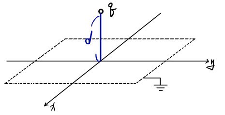
The boundary conditions are basically all set.

What the boundary conditions were — the potential values at the boundary were the boundary conditions.

Then, the boundaries would be the very bottom and the very top! — but…

You might ask: the very bottom has a conductor plane so there’s a boundary, but there’s no boundary at the top,

but if we go infinitely in the z-axis direction, V=0, right?

Because we get super far from q, so we say the boundaries are set

Let me write the boundary conditions.

1. When z=0, V=0

2. When z=infinity, V=0

Since we know all the boundary conditions, we can know all the potentials inside the boundary!

(This was the ‘uniqueness theorem’!! (which tells us GD, what you found is unique^^))

Editor’s note — 2 October 2026. The full boundary problem also specifies the real point charge and its Coulomb singularity. The potential must approach zero at spatial infinity in every direction within the upper region, not only when moving up the z-axis. Uniqueness applies with these source and boundary conditions fixed; the point occupied by the charge is excluded from the ordinary field region.

Now then, the potential at any point above the plane won’t be the

‘one over four pi epsilon zero times q over r’ that we’ve been using up till now

Because due to q, induced charges appear on the conductor plane,

and near q there’s a somewhat large induced charge, and far away there’s a small induced charge!!

(The induced charges would also be induced in a crazy complicated way, right? Because on the plane close to q a correspondingly large charge will be induced, and on the plane far away a relatively small charge will be induced.)

In this case, we can use the image method. It’s a trick to solve the problem a bit easily, a trick.

What the trick is — we bring in a few imaginary charges to create the situation the problem demands!

Alright! Let’s remove the grounded conducting plane for just a moment, and put a -q charge at z=-d

Because intuitively it feels like doing that would match the boundary conditions the same way

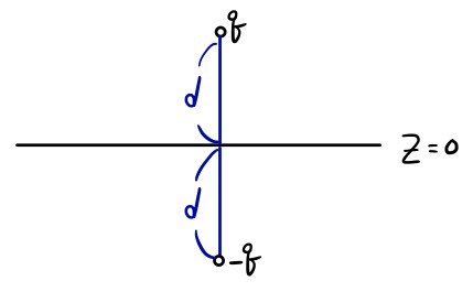
Let’s compute V(x,y,z) and check whether V=0 at z=0 for real

It’d be the potential due to -q + the potential due to q

Plugging 0 into z gives V(x,y,0) = 0

and plugging infinity into z gives 0

We succeeded in placing imaginary charges that produce the same boundary conditions with a new situation!

Then, in that situation with the imaginary charge placed, if we look only at the region z≥0, that’s the situation of our problem!!!

And the “uniqueness theorem” guarantees that this solution is the unique solution.

What was the logic of the uniqueness theorem — if it satisfies the Poisson equation and

satisfies the values at the boundary, that’s the unique solution! That’s what it was~~~

Therefore~ done! The problem is all solved!!

Alright, but since we’re in the position of studying, let me find more from that situation.

Since E=-∇V, if we partial-differentiate V with respect to x, y, z and compute (having summed them), how does it go

Everything that would cancel out cancels and flies away, and what remains is

Editor’s note — 2 October 2026. The transverse field components cancel on the conducting plane, not throughout the space above it. The historical equation linked next also has the opposite sign for its z component. Keep this equation as a historical source reference; the corrected three-component field is derived in “Differentiate to find the electric field” below.

View the original historical field-expression image. The source expression gives only a z component and has a sign error; the reviewed derivation below supplies all three corrected field components.

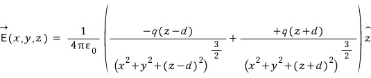
What if you’re also curious about the charge density ρ(x,y) on the plate? hehe

We’d need to bring the plate back for a moment, right, since we’re curious about the charge density on the plate?

Take a Gaussian surface on the plate lollol how we take a Gaussian surface on a plate is — we take a (freakin’ tiny) cylinder.

View the original historical two-sided pillbox diagram. This is the original diagram discussed in the note. A conductor pillbox has zero interior field; the reviewed derivation below distinguishes it from the two-sided sheet construction.

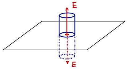
Like this! The electric field due to the charge density on the plate all cancels out and only the perpendicular direction remains!

So if we apply Gauss’s law there, let me call the base area of the Gaussian cylinder dA (freakin’ tiny A).

2(dA)|E| = Qin/ε = ρ(dA)/ε

|E| = ρ/2ε

E = (ρ/2ε)z

Then the relationship between ρ and E at the surface of this situation is εE = ρ

Editor’s note — 2 October 2026. The preceding algebra mixes two boundary problems and drops a factor of two when it moves to the final relation. For the total field at a conductor surface, the lower pillbox face is inside the conductor and has zero field, so only the upper face contributes. The signed normal field just outside is the surface charge density divided by the vacuum permittivity. The two-sided factor of two belongs to a free sheet construction. The original note calls the surface density rho; the reviewed derivation calls it sigma. Tangential cancellation at the conductor surface concerns the total field, including the real charge, rather than the induced-charge field alone at every position.

So since that’s it, we found E earlier

if we just multiply by ε, wouldn’t that do it?

Ah@@@ and since our ρ we found must be defined only at z=0! we mustn’t forget to plug 0 into z

View the original historical surface-density equation. The source image has exponent 2/3. The corrected conductor surface density with exponent 3/2 is derived in the reviewed section below.

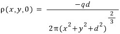
As expected, the (‘induced’) charge density is large at (0,0,0) ~

Editor’s note — 2 October 2026. For a positive real charge, the induced density is negative. “Large” here means greatest in magnitude beneath the charge, not the largest signed numerical value. The historical density image linked above prints the denominator exponent as two thirds; the correct exponent is three halves, as derived below.

And also, if we integrate over the infinite plane, we get -q, which would also be obvious, right?

Since it’s the collection of induced charges generated by +q, a total of -q would be induced.

Editor’s note — 2 October 2026. The total induced charge equals minus q for this infinite grounded plane. It follows by integrating this geometry’s surface density. It is not a general consequence of induction on an arbitrary conductor; grounding permits exchange of charge with a reservoir.

I’m just gonna milk this problem for all it’s worth.

The +q charge would be subject to a force due to the charges induced on the conductor plate, right?

How much force is exerted?

Same thing. Remove the plate, put -q at position -d, and calculate.

So

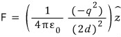
Editor’s note — 2 October 2026. This is the force from the induced charges, represented by the image charge. Exclude the real point charge’s singular self-field. The force points toward the plane for either sign of the real charge.

What about the energy, the energy?

“When using the image method, you have to be careful with the energy!!! Because”

It’s when our newly constructed imaginary space becomes a different space from the actual (in-the-problem) one.

So

the energy when the plate and q are there would be half of the energy when there are two charges, right?

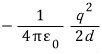
When there are two charges it’d be

but

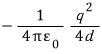
when the plate and q are there, half of that,

it’d be.

Editor’s note — 2 October 2026. These are finite interaction energies with the point charges’ divergent self-energies excluded. The half-factor shown here compares this grounded-plane system with the two-real-charge system at the displayed separation. Matching fields in the upper region alone does not justify equating assembly energies: the conductor’s induced charge and the image position change as the real charge moves. The quasistatic work calculation below gives the plane result without assuming a half-factor for every image geometry.

In the image method, the energy in particular is something to be careful with

Image method end~

Reviewed scientific explanation

The following English scientific edition and its dated editorial correction are preserved in full.

The method of images turns a conductor problem into a charge problem that we can solve directly. We choose imaginary charges to reproduce the required boundary potential, then use uniqueness to justify the construction. Once we know the potential, differentiation gives the electric field:

$$ \mathbf E=-\nabla V. $$

The minus sign matters. Each field component is the negative partial derivative of the potential along that coordinate.

The boundary problem

Place a fixed point charge $q$ at $(0,0,d)$, with $d>0$, in vacuum above an infinite ideal conducting plane at $z=0$. The plane is grounded: its potential stays at zero, and charge can flow between the conductor and a reservoir.

Refer to the original narrative image: Point charge q at height d above a grounded conducting plane in the x-y plane.

We want the potential in the upper region, $z>0$, excluding the point occupied by the charge. Its boundary value on the plane is

$$ V(x,y,0)=0. $$

We also require $V$ to approach zero at spatial infinity in every direction within the upper region. Letting only $z$ grow would not state the full condition. The source is specified too: the potential must have the Coulomb singularity of charge $q$ at $(0,0,d)$ and no other singularity above the plane.

The induced surface charge is initially unknown, so the isolated-charge potential is not enough. The image construction gives us a way to include its effect without first finding that charge distribution. Whether a useful construction exists depends on the boundary geometry; a simple finite set of images is not available for an arbitrary conductor.

Choose an image and check the potential

For the auxiliary charge problem, remove the conductor and put an image charge $-q$ at $(0,0,-d)$. The real charge and its image are equally far from the plane.

Refer to the original narrative image: Real charge q at z equals d and image charge minus q at z equals minus d, reflected across z equals zero.

Define the Coulomb constant and the distances from an observation point to the two charges:

$$ k=\frac{1}{4\pi\epsilon_0}, $$$$ R_+=\sqrt{x^2+y^2+(z-d)^2}, $$$$ R_-=\sqrt{x^2+y^2+(z+d)^2}. $$

Adding the two Coulomb potentials gives the expression in the original equation image:

Refer to the original narrative image: Potential above the plane: Coulomb potential of q at height d plus that of the image charge minus q at height minus d.

In the shorter notation, this is

$$ V=kq\left(\frac{1}{R_+}-\frac{1}{R_-}\right). $$

On the plane, the two distances are equal, so the terms cancel. At spatial infinity both terms tend to zero. In the upper region, the image contribution is nonsingular, and the real-charge term has exactly the required source singularity.

These checks make the construction a solution of the boundary problem. To see why it is the unique decaying solution, subtract it from any other solution with the same charge singularity and boundary values. The singularities cancel; the difference extends to a harmonic function with zero boundary values and decay at infinity. The uniqueness theorem then makes that difference zero.

The image charge lies outside the physical region we are solving. Continuing this formula below the plane does not give the field inside the conductor or in the shielded lower region. The actual conductor is equipotential, and its electrostatic interior field is zero.

Differentiate to find the electric field

Keep all three components when taking the negative gradient. Away from the real charge, in the upper region,

$$ E_x=kqx\left(\frac{1}{R_+^3}-\frac{1}{R_-^3}\right), $$$$ E_y=kqy\left(\frac{1}{R_+^3}-\frac{1}{R_-^3}\right), $$$$ E_z=kq\left(\frac{z-d}{R_+^3}-\frac{z+d}{R_-^3}\right). $$

The vector field is assembled from these components:

$$ \mathbf E=E_x\hat{\mathbf x}+E_y\hat{\mathbf y}+E_z\hat{\mathbf z}. $$

The transverse components generally remain nonzero above the plane. On $z=0$, however, equal distances make both $E_x$ and $E_y$ vanish. The field immediately outside the conductor is therefore normal to its surface, as an electrostatic conductor requires.

Find the induced surface charge

Use $\sigma$ for charge per unit area; $\rho$ would denote charge per unit volume. To relate $\sigma$ to the field, imagine a thin Gaussian pillbox straddling the surface. Its lower face lies inside the conductor, its upper face lies just outside, and the outward normal from the conductor is $\hat{\mathbf n}=\hat{\mathbf z}$.

In the thin limit, the side flux vanishes. The upper and lower faces have opposite outward normals, so Gauss’s law gives

$$ (\mathbf E_{\rm out}-\mathbf E_{\rm in})\cdot\hat{\mathbf n} =\frac{\sigma}{\epsilon_0}. $$

Here $\mathbf E_{\rm in}=0$. Only the upper face contributes, giving

$$ \sigma=\epsilon_0 E_z(0^+). $$

There is no factor of two from the two faces. A free sheet with equal fields on both sides is a different boundary problem; it does not describe this conductor pillbox.

Evaluate the field from above at $z=0$:

$$ E_z(x,y,0^+)= -\frac{qd}{2\pi\epsilon_0(x^2+y^2+d^2)^{3/2}}. $$

Thus the induced density is

$$ \sigma(x,y)= -\frac{qd}{2\pi(x^2+y^2+d^2)^{3/2}}. $$

For a positive $q$, the field just outside points toward the conductor and the induced surface charge is negative. Its magnitude is greatest directly beneath the charge and decreases with distance along the plane. The exponent is $3/2$, giving the required dimensions of charge per area.

Integrate over the plane

Write the distance from the axis as $s=\sqrt{x^2+y^2}$. A circular ring has area $2\pi s\,ds$, so the charge within radius $R$ is

$$ Q(R)=\int_0^R\sigma(s)\,2\pi s\,ds, $$$$ Q(R)=-qd\int_0^R\frac{s\,ds}{(s^2+d^2)^{3/2}}. $$

Using the antiderivative $-1/\sqrt{s^2+d^2}$ yields

$$ Q(R)=\frac{qd}{\sqrt{R^2+d^2}}-q. $$

Taking the radius to infinity gives

$$ Q_{\rm induced}=-q. $$

The equality follows from this infinite grounded-plane geometry. It is not a general rule that every conductor near a charge acquires the opposite total charge. Grounding allows the exchange with a reservoir needed to maintain the prescribed potential.

Force on the real charge

The force on $q$ comes from the induced charges. Exclude the singular self-field of the real point charge. In the image construction, the induced field at the real charge is simply the field of $-q$, a distance $2d$ away.

Refer to the original narrative image: Force on the real charge: minus q squared divided by sixteen pi epsilon zero d squared, directed along the positive z unit vector with a negative coefficient.

The equivalent expression is

$$ \mathbf F=-\frac{q^2}{16\pi\epsilon_0d^2}\hat{\mathbf z}. $$

The force points toward the plane for either sign of $q$. Changing the charge’s sign also reverses the induced charge, leaving the attraction unchanged.

Why the energy needs a separate calculation

Two independently real charges $q$ and $-q$, separated by $2d$ in vacuum, would have the following interaction energy:

Refer to the original narrative image: Interaction energy of two real opposite charges separated by twice d: minus q squared divided by eight pi epsilon zero d.

$$ U_{\rm pair}=-\frac{q^2}{8\pi\epsilon_0d}. $$

This excludes the divergent self-energies of the individual point charges. It describes a physical two-charge system, whereas our actual system contains one point charge and a grounded conductor. Matching the field in the upper region does not make these two systems’ assembly energies equal.

Bring the charge in from infinity

Move $q$ slowly along the axis toward the grounded plane. At a temporary height $a$, the electric force component is

$$ F_z(a)=-\frac{q^2}{16\pi\epsilon_0a^2}. $$

An external agent balances this force during quasistatic motion, with no change in kinetic energy. Set the distance-dependent interaction energy to zero at infinity. The external work is then

$$ U(d)=-\int_{\infty}^{d}F_z(a)\,da, $$$$ U(d)=\frac{q^2}{16\pi\epsilon_0}\int_{\infty}^{d}\frac{da}{a^2}, $$$$ U(d)=-\frac{q^2}{16\pi\epsilon_0d}. $$

This agrees with the original grounded-plane energy image:

Refer to the original narrative image: Interaction energy of a point charge and grounded plane: minus q squared divided by sixteen pi epsilon zero d.

The negative work means the external agent removes energy while lowering the charge under control. Another way to express the same result uses the induced potential at the real charge:

$$ V_{\rm induced}(0,0,d)=-\frac{q}{8\pi\epsilon_0d}, $$$$ U(d)=\frac{1}{2}qV_{\rm induced}(0,0,d). $$

As the charge moves, the induced charges readjust and the image position changes with it. The image is not an independently fixed physical charge. Differentiating $U_{\rm pair}(d)$ would count a different motion of a different system and give the wrong force for the grounded-plane problem. The numerical half-factor between these two displayed energies belongs to this plane construction; it should not be assumed for every image geometry.

Throughout this calculation, $U$ is the finite interaction or assembly energy with the point charge’s infinite self-energy excluded. It is not the unregularized integral of the nonnegative total field energy density over all space. Calculating the external work keeps that distinction explicit while respecting the grounded boundary.

The image construction has now given us the potential, field, surface charge, and force. For energy, the essential extra step was to follow the actual grounded system as the charge moved.

Refer to the original narrative image: Decorative character sticker from the original study note; no scientific information.

Editorial correction

Editorial correction — 2026-09-09. This English edition of the original study note restores the potential equation that had been replaced by a misplaced pillbox image. It replaces the historical field-expression image, two-sided pillbox diagram, and surface-density image with corrected typeset mathematics and explanation. Those historical source files are preserved.

The corrections include the negative gradient and all three field components, the conductor pillbox with zero interior field, and the surface-density exponent $3/2$. The text also makes the spatial boundary and charge-singularity conditions explicit, and derives the grounded-plane energy from quasistatic work with point-charge self-energy excluded. The retained force and energy images agree with the expressions explained here.

For further derivations, see the University of Texas at Austin notes on the method of images and ideal conductors.