Multipole expansion: the original learning narrative

I wrote this learning note on 17 November 2014. The English narrative follows the original order; dated editorial notes identify scientific qualifications and source formula corrections. A complete scientific appendix follows.

Original Korean learning note

Far away, does a charge distribution look like a point charge?

What is a multipole expansion?

I have only just learned about it myself, but it seems quite interesting!

Suppose there is a “charge distribution” somewhere, and we look at it from a ridiculously long way away.

From very, very far away, that whole collection of charges looks like a point charge.

We might think, “Huh? Is that little thing over there a point charge?” and calculate its potential.

Even if we use the familiar formula \(V(r)=Q/(4\pi\epsilon_0 r)\),

we get an approximately right answer.

Editorial qualification — 2 October 2026. The distant point-charge intuition assumes a nonzero total charge for a leading monopole term; neutral distributions need their first nonzero higher moment.

Let me try to explain why it is approximately right!

Start with a dipole

First,

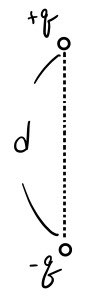
let us look at this case. I chose it deliberately because it is related to an electric dipole.

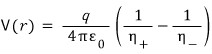
Shall we find the potential from a very, very distant point?

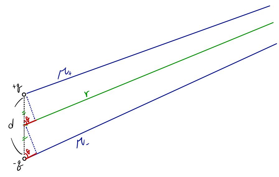
I will use these variables to make an approximation.

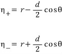
Writing the relative distances in terms of r gives the following.

Original source formula 5 — Historical source formula: subtraction of the two projected inverse distances, followed by the far-field dipole potential. The source prints a plus sign in the denominator where the algebra requires a minus sign.

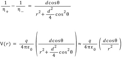
Source correction — 2 October 2026. The projected distances are approximations, and their denominator is r squared minus (d squared/4) cos squared(theta). The corrected derivation is preserved in the scientific appendix.

We can make an approximation like this.

To sum up: if there is a monopole contribution, its potential is inversely proportional to distance.

For the dipole we just looked at, we can approximate the potential as inversely proportional to distance squared.

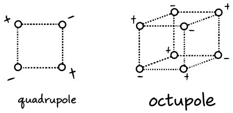
For a quadrupole like this, the potential at distance r is approximately inversely proportional to r cubed.

For an octupole, the potential at distance r is approximately inversely proportional to the fourth power of r.

Editorial qualification — 2 October 2026. These inverse powers describe the leading potential at directions where its angular factor is nonzero. Finite square and cube examples require equal-magnitude charges in centered symmetric positions, and may also contain higher moments.

A more general charge distribution

Now let us do something more general than the example above, which was quite openly about a dipole!

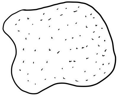
Suppose charges are crowded together in a region like this. Let us estimate the potential a distance r away.

We add up the potential contributions from every little piece of volume charge density, one by one.

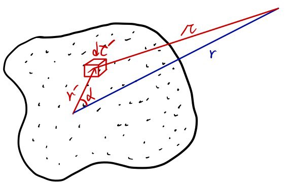
If we define the variables this way, we get the following expression.

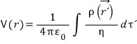
Here again, we can express the relative distance

in terms of r, using the law of cosines we learned in high-school mathematics.

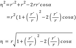
Original source formula 11 — Historical source formula and aside: “I will rewrite 1/R as (1/r)/sqrt(1+epsilon) for a moment, because I want to use the binomial theorem.” The image shows the coefficients 1, -1/2, 3/8, -5/16, and further terms.

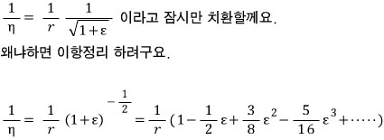
Source correction — 2 October 2026. Use epsilon = t squared - 2t cos(alpha), where t=r-prime/r. The inverse-square-root binomial coefficients shown here are correct. The full Legendre expansion has exterior domain r-prime < r; the intermediate binomial series has its own convergence condition, and collecting the cubic term requires the displayed -5 epsilon cubed/16 term. See the appendix for the domain and termwise-integration qualification.

I think that in high-school mathematics we only dealt with natural-number powers, so I actually had to look up a case like this myself!

Did we do it when we studied Taylor series? I feel as though I have seen it somewhere before…

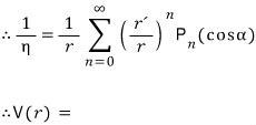
The source image ends with a “therefore V(r) =” lead-in; the potential expansion is continued below.

Now there is a slightly tedious calculation to do: sort the terms inside the braces by powers of \((r\prime/r)\).

I tried working it out roughly myself…

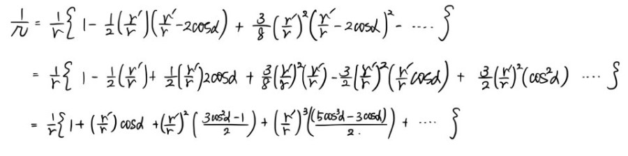
Source correction — 2 October 2026. The last handwritten line has the correct cubic Legendre coefficient, but the displayed intermediate steps do not show the contribution from -5 epsilon cubed/16, with epsilon = t squared - 2t cos(alpha). Those steps alone do not establish the cubic coefficient; that omitted contribution must be included when collecting powers of t. The complete generating-function derivation is preserved in the appendix.

My conclusion was that “\((r\prime/r)^n\) is a coefficient of the Legendre polynomials.”

Editorial qualification — 2 October 2026. The original sentence describes the coefficient relationship loosely. Precisely, the coefficient of t to the power n is P_n(cos alpha), with t=r-prime/r; the powers themselves are not coefficients of the Legendre polynomials.

(To be honest, I have not learned Legendre polynomials in mathematics class yet.

In electromagnetism class, I am just accepting that this is how it works for now.

When I have time, I think I should study that part properly. Legendre polynomials seem to come up quite often in electromagnetism!)

Original source formula 14 — Historical source formula: insert the Legendre series into the potential integral and “expand out the sum.” The source uses r-prime squared in the general term, then an incorrect cubed radius and unsquared cosine in the quadrupole term.

Source correction — 2 October 2026. The general integrand needs r-prime to the order n. The quadrupole factor needs r-prime squared times (3 cos squared(alpha)-1)/2. The corrected expressions are given in the appendix.

What this broken-down, expanded expression tells us is this:

if we look at a collection of charges from far, far away and calculate the potential at that distant point,

we can express it as a sum of the potentials due to monopole, dipole, quadrupole, and further contributions!

Also, alpha is the angle between r and r-prime, so it changes with the position of r, does it not?

That means the expansion as we see it can also depend on where we look from!

Editorial qualification — 2 October 2026. Moving the observer changes r and the angular factors at which fixed source moments are evaluated. With a fixed source and origin, it does not change the source moments themselves.

(For the actual dipole we used right at the beginning, the monopole and quadrupole contributions, among others, were zero.)

Editorial qualification — 2 October 2026. A centered finite +q,-q pair is inversion-odd: all even orders cancel, while odd orders beyond the dipole may remain.

And the farther away r is, the closer the higher-order terms, such as the quadrupole and octupole terms, get to zero. In that sense the monopole and dipole terms can be the important ones.

Another point: if we choose the z-axis parallel to the direction of r, alpha becomes the polar angle in spherical coordinates, making the calculation easier.

(An approximation along the z-axis looks manageable, at least!)

Editorial qualification — 2 October 2026. Here alpha is the source polar angle theta-prime when the z-axis is along the observer direction. In the final dipole-field calculation, theta is instead the observation angle with the z-axis along p.

Pick out the dipole term

Let us follow that intuition a little farther. Usually, when the total charge Q is nonzero, the monopole term in the multipole expansion is the largest one—provided r is enormously large.

When the total charge is zero, the largest term is the dipole term.

(Of course, that assumes the dipole integral is not zero! Higher-order terms scale as one over r cubed, one over r to the fourth, and so on, so they die away faster than the dipole term.)

Translation note — 2 October 2026. The source uses a malformed four-pole comparison term in this sentence. “Dipole term” above is a marked contextual repair of that wording. The corrected comparison is that nonzero quadrupole and octupole potentials decay as one over r cubed and one over r to the fourth, faster than the dipole potential, away from angular nodes.

Editorial qualification — 2 October 2026. The leading radial order is the lowest nonzero moment away from its angular nodes. A zero potential at a node does not imply a zero field.

Let us pick out just the dipole term.

Original source formula 15 — Historical source formula: isolate the dipole term, use the projection r-prime dot r-hat = r-prime cos(alpha), and factor the observation-direction unit vector outside the integral. The final expression does not visibly mark the required dot product.

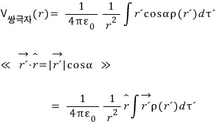
Source correction — 2 October 2026. The dipole potential is a scalar; the final contraction requires an explicit dot product. The appendix keeps the corrected vector notation.

Looking at the integral, we multiply a vector by the scalar charge density rho and add those contributions throughout the volume. After adding them all, we get one vector, right?

We will call that resulting vector the “electric dipole moment.”

Original source formula 16 — Historical source formula: define the dipole moment as the volume integral of source-position vector times charge density, and write the dipole potential as p dot r-hat divided by 4 pi epsilon-zero r squared.

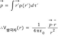
Now we can express the potential in this form!

For n charges gathered together, we can write their dipole moment as the following sum.

Return to the two-charge dipole

Now let us go back to the dipole made of -q and +q.

I will try to make the identity of the vector p clear once more.

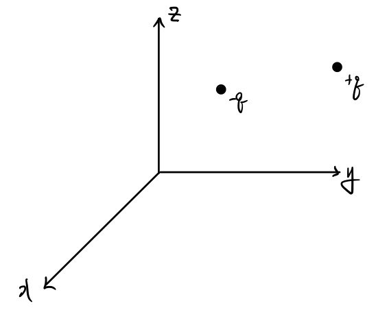
Suppose +q and -q are located somewhere in this coordinate space.

Then

let r-prime-1 be the vector from the origin to -q,

and r-prime-2 the vector from the origin to +q.

The vector from -q to +q is therefore minus r-prime-1 plus r-prime-2.

Let us call that vector d.

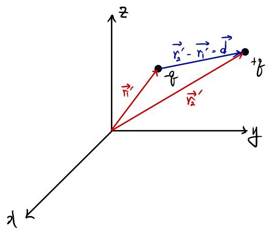
Like this.

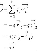
What if the dipole moment is zero too?

So if the total charge is zero, is the dipole term always the largest one?

No! We already assumed that the dipole term itself was nonzero, remember?

Then when can the total charge be zero and the dipole term also be zero?

A simple example is a quadrupole. Its dipole term is zero.

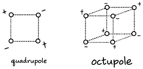
Take a look at the quadrupole, whichever way you group the charges.

You get two dipole-moment vectors, do you not? They point up and down, or right and left.

The vector sum of those individual dipole moments gives the total dipole moment, just as in the sum of q-i times r-i we wrote earlier.

So in this case the dipole term is zero, and the quadrupole term determines the leading potential in the multipole expansion.

Editorial qualification — 2 October 2026. For the centered equal-magnitude square, its two equal and opposite pair dipole moments cancel. The leading quadrupole may coexist with higher moments; its angular factor can vanish along particular directions.

Where did we put the origin?

There is another important point about multipole expansions:

“Where is the origin of the coordinate system?”

For example,

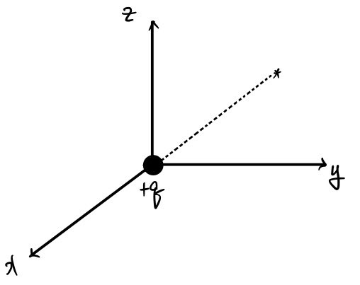
when a charge +q sits at the coordinate origin, is the dipole term in its potential at r zero?

Why is it zero?

In the definition below, the source-position vector r-prime is zero, so the dipole term is zero.

But here is something interesting!

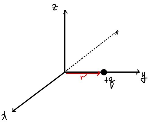
If the charge +q is away from the origin, its source-position vector r-prime survives.

That means a dipole term survives too.

The point I want to make is that the multipole expansion can depend on where we put the coordinate origin!

Earlier, the expression for the same charge distribution depended on where r was, remember? I think we can look at this in a similar spirit.

Editorial qualification — 2 October 2026. These are distinct effects: observer changes alter the evaluation point; origin shifts alter moment coordinates. Under an origin shift a, p-new = p-old - Q a, and the full physical potential and field remain invariant when transformed consistently.

The dipole electric field

Finally, let us look at the electric field produced by a dipole. We will use the fact that the field is minus the gradient of V.

Editorial qualification — 2 October 2026. For the finite pair of charges discussed above, keeping only the dipole term gives the leading far-field potential and field; it is not the full finite-separation result. For an ideal point dipole, the dipole formulas are exact at r>0. In this final section the z-axis is chosen along the dipole moment, and theta is the observation angle.

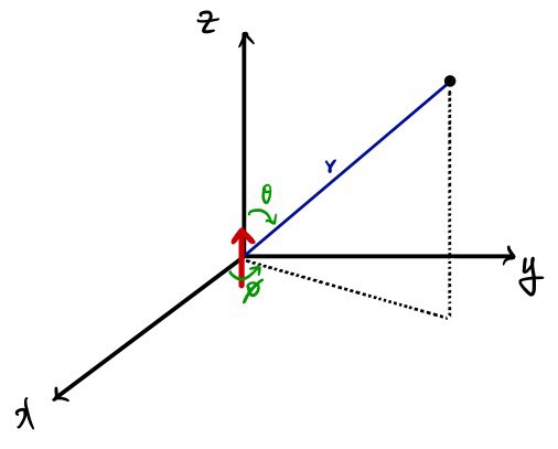
Earlier, we found this expression.

Original source formula 26 — Historical source formula: write the dipole potential first as p dot r-hat divided by 4 pi epsilon-zero r squared, then as p cos(theta) divided by the same denominator.

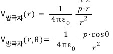
It does not depend on phi.

Now let us take the gradient.

Original source formula 27 — Historical source formula: apply minus the gradient to the dipole potential in spherical coordinates. Its first radial component omits p, while the final factored line includes p.

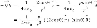
Source correction — 2 October 2026. The radial component needs the same factor p as the polar component. The ideal-dipole expression applies for r>0. The appendix includes the corrected field.

That is the end of the multipole expansion!

---

Scientific appendix: corrected derivation and qualifications

This preserves the previously reviewed scientific explanation. Diagram links point back to their original occurrences in the narrative above.

What is a multipole expansion?

I had just encountered it when I wrote the original post, and the basic idea is surprisingly intuitive. A localized charge distribution viewed from far away can often be described by a sequence of progressively finer terms: monopole, dipole, quadrupole, and so on. If the total charge is nonzero, the monopole term usually dominates the far field. If it vanishes, the first nonzero higher moment takes over.

Starting with a finite dipole

Consider two charges, \(+q\) and \(-q\), separated by a displacement of magnitude \(d\).

See source diagram 1: Two opposite charges, plus q and minus q, separated by distance d

Place the charges at \(\pm (d/2)\hat{\mathbf z}\), and let the observation point be \(\mathbf r\), with \(r=|\mathbf r|\) and polar angle \(\theta\).

See source diagram 2: Far-field geometry for a centered electric dipole, showing r, d, theta, and source distances

The exact potential is the sum of the two point-charge potentials:

See source diagram 3: Exact potential of the two-charge dipole in terms of the two source distances

The exact source-to-field-point distances are

\[ R_+=\sqrt{r^2+\frac{d^2}{4}-rd\cos\theta}, \qquad R_-=\sqrt{r^2+\frac{d^2}{4}+rd\cos\theta}. \]

For \(r\gg d\), their first-order projected-distance approximations are

See source diagram 4: First-order far-field approximations for the two source distances

or \(R_+\approx r-(d/2)\cos\theta\) and \(R_-\approx r+(d/2)\cos\theta\). Substituting these approximations gives

\[ \begin{aligned} V(r,\theta) &\approx \frac{q}{4\pi\epsilon_0} \left[ \frac{1}{r-(d/2)\cos\theta} -\frac{1}{r+(d/2)\cos\theta} \right] \\ &=\frac{1}{4\pi\epsilon_0} \frac{qd\cos\theta}{r^2-(d^2/4)\cos^2\theta} \\ &\approx \frac{1}{4\pi\epsilon_0}\frac{p\cos\theta}{r^2}, \qquad p=qd, \end{aligned} \]

where the last line keeps the leading term for \(r\gg d\).

Source correction. The source image at this point prints a plus sign in the projected-distance denominator. The corrected denominator is \(r^2-(d^2/4)\cos^2\theta\), as shown above.

The pattern is now visible. A monopole contribution scales as \(r^{-1}\), a dipole contribution as \(r^{-2}\), a quadrupole contribution as \(r^{-3}\), and an octupole contribution as \(r^{-4}\). These statements describe the radial order at a fixed direction where the relevant angular factor is nonzero. An angular node of the potential does not mean that the whole multipole moment—or even the electric field—vanishes there.

See source diagram 6: Alternating-charge quadrupole and octupole arrangements

For the centered \(+q,-q\) pair above, inversion symmetry makes the charge distribution odd. Its even-\(\ell\) contributions cancel, but odd orders beyond the dipole, such as \(\ell=3,5,\ldots\), can still remain. Calling it a “dipole” identifies its leading nonzero moment, not the only term in the exact finite-separation potential.

A general localized charge distribution

Now consider a continuous charge distribution confined to a finite region.

See source diagram 7: Localized continuous charge distribution

Let \(\mathbf r\) be the observation point and \(\mathbf r'\) a source point. Define

\[ \mathbf R=\mathbf r-\mathbf r',\qquad R=|\mathbf R|,\qquad r=|\mathbf r|,\qquad r'=|\mathbf r'|, \]

and let \(\alpha\) be the angle between \(\mathbf r\) and \(\mathbf r'\), so that \(\cos\alpha=\hat{\mathbf r}\cdot\hat{\mathbf r}'\).

See source diagram 8: Source point and observation point geometry for a continuous charge distribution

The electrostatic potential is

See source diagram 9: Coulomb-potential integral for a continuous charge density

and the geometry gives

See source diagram 10: Law-of-cosines expression for the source-to-field-point distance

that is,

\[ R^2=r^2+r'^2-2rr'\cos\alpha. \]

Set \(t=r'/r\). The Legendre generating function gives

\[ \frac{1}{R} =\frac{1}{r}\left(1-2t\cos\alpha+t^2\right)^{-1/2} =\frac{1}{r}\sum_{\ell=0}^{\infty}t^\ell P_\ell(\cos\alpha), \qquad r'\lt r. \]

For a source contained inside \(r'\le a\), this exterior expansion applies for \(r>a\). On any region \(r\ge r_0>a\), the series converges uniformly enough to justify term-by-term integration.

If one reaches the result through the binomial series, it is important not to stop too soon. With \(u=t^2-2t\cos\alpha\), a derivation through \(P_3\) needs the \(-5u^3/16\) term; the displayed \(u^0\), \(u^1\), and \(u^2\) terms alone do not produce the full cubic coefficient. The Legendre generating function is also the clean way to state the full domain \(|t|<1\); the intermediate condition \(|u|<1\) can be unnecessarily restrictive.

See source diagram 12: Legendre generating series for the inverse source-to-field-point distance

The first few terms are

See source diagram 13: Collected expansion through the first four Legendre polynomials

so the coefficient of \(t^\ell\) is \(P_\ell(\cos\alpha)\). Substituting the series into the potential produces

\[ V(\mathbf r) =\frac{1}{4\pi\epsilon_0} \sum_{\ell=0}^{\infty}\frac{1}{r^{\ell+1}} \int r'^\ell P_\ell(\cos\alpha)\rho(\mathbf r')\,d\tau'. \]

The first three orders are

\[ V(\mathbf r)=\frac{1}{4\pi\epsilon_0} \left[ \frac{Q}{r} +\frac{1}{r^2}\int r'\cos\alpha\,\rho(\mathbf r')\,d\tau' +\frac{1}{r^3}\int \frac{r'^2}{2}\left(3\cos^2\alpha-1\right) \rho(\mathbf r')\,d\tau' +\cdots \right], \]

with \(Q=\int\rho(\mathbf r')\,d\tau'\).

Source correction. The source image uses \(r'^2\) in the general \(\ell\) term and gives an incorrect power and angular factor in the quadrupole term. The equations above restore \(r'^\ell\) generally and \(r'^2(3\cos^2\alpha-1)/2\) at \(\ell=2\).

For a fixed source distribution and a fixed origin, the multipole moments are fixed. Moving the observer changes \(r\) and the angular factors at which the expansion is evaluated; it does not change the source moments themselves. If the \(z\)-axis is chosen along \(\mathbf r\), then \(\alpha\) is the source point’s polar angle \(\theta'\). Later, when the \(z\)-axis is chosen along \(\mathbf p\), the \(\theta\) in \(p\cos\theta\) is the observation angle. Those are different coordinate choices.

The far-field hierarchy is controlled by the lowest nonzero moment, but only away from its angular nodes. When \(Q\ne0\), the monopole term is normally leading. When \(Q=0\), the dipole term leads only if the dipole moment is nonzero.

The dipole moment

The dipole term can be written using

\[ \mathbf p=\int \mathbf r'\rho(\mathbf r')\,d\tau', \qquad V_{\mathrm{dip}}(\mathbf r) =\frac{1}{4\pi\epsilon_0}\frac{\mathbf p\cdot\hat{\mathbf r}}{r^2}. \]

Source correction. The corresponding source image omits the explicit scalar-product dot in its last expression. It is restored here because the potential is a scalar.

For discrete point charges,

See source diagram 17: Electric dipole moment of discrete point charges

or \(\mathbf p=\sum_i q_i\mathbf r_i'\).

Return to a pair of charges \(-q\) and \(+q\).

See source diagram 18: Two opposite point charges in Cartesian coordinates

Let \(\mathbf r_1'\) point from the origin to \(-q\), and \(\mathbf r_2'\) point from the origin to \(+q\). Define the displacement from the negative charge to the positive charge by

\[ \mathbf d=\mathbf r_2'-\mathbf r_1'. \]

See source diagram 19: Dipole displacement vector from minus q to plus q

Then

See source diagram 20: Derivation of p equals q times d for two opposite charges

so \(\mathbf p=q\mathbf d\).

When the dipole moment also vanishes

A neutral distribution need not have a nonzero dipole moment. With equal-magnitude charges at centered symmetric positions, an alternating-charge square has \(Q=0\) and \(\mathbf p=0\), while a quadrupole component remains. Likewise, the centered alternating cube shown below cancels all orders below \(\ell=3\), leaving an octupole as its leading moment. Finite arrangements can still contain higher moments beyond the leading one.

See source diagram 21: Centered alternating-charge quadrupole and octupole examples

This is why “the first nonzero multipole” is the useful phrase: symmetry may eliminate one or several lower orders.

Dependence on the choice of origin

There is one more important detail: multipole moments are coordinates of a source relative to a chosen origin.

See source diagram 22: Single point charge located at the coordinate origin

For a point charge at the origin, the discrete definition

See source diagram 23: Discrete dipole-moment definition applied at the origin

gives zero dipole moment.

See source diagram 24: Single point charge displaced from the coordinate origin

If the origin is shifted by a vector \(\mathbf a\), so that \(\mathbf r'_{\mathrm{new}}=\mathbf r'_{\mathrm{old}}-\mathbf a\), then

\[ \mathbf p_{\mathrm{new}}=\mathbf p_{\mathrm{old}}-Q\mathbf a. \]

Therefore the dipole moment is origin-independent when \(Q=0\), but not in general. This coordinate dependence of individual moments does not change the physical potential or electric field when the whole expansion and coordinates are transformed consistently.

Electric field of an ideal dipole

Choose the \(z\)-axis along \(\mathbf p=p\hat{\mathbf z}\), and use spherical coordinates for an observation point away from the source.

See source diagram 25: Spherical coordinates for an observation point relative to the dipole axis

For \(r>0\), the ideal-dipole potential is

\[ V_{\mathrm{dip}}(r,\theta) =\frac{1}{4\pi\epsilon_0} \frac{\mathbf p\cdot\hat{\mathbf r}}{r^2} =\frac{1}{4\pi\epsilon_0}\frac{p\cos\theta}{r^2}. \]

It is independent of the azimuthal angle \(\phi\). Taking \(\mathbf E=-\nabla V\) gives

\[ \mathbf E(r,\theta) =\frac{p}{4\pi\epsilon_0 r^3} \left(2\cos\theta\,\hat{\mathbf r} +\sin\theta\,\hat{\boldsymbol\theta}\right), \qquad E_\phi=0, \qquad r>0. \]

Source correction. The source image omits \(p\) from its first displayed radial component. The corrected field above includes it. The ideal-dipole expression is not defined at \(r=0\).

That completes the basic picture: expand the inverse distance in Legendre polynomials, integrate each angular order against the source, and let the first nonzero moment describe the leading far field.

References

• MIT OpenCourseWare 8.07, Lecture Notes 9: Legendre polynomials, spherical harmonics, and multipole expansion
• University of Illinois Physics 435, Lecture 8: Electric dipoles and fields
• Original Korean post