Separation of Variables: Strips and Pipes

Original study note — faithful English narrative

Read the reviewed scientific explanation.

Source narrative restored (2 October 2026). This edition preserves the complete original note of 17 November 2014, including its jokes, personal ending, and linked-post card. Historical terminology and mathematical errors are attributed to the original note. Seven historical source images are linked with full English context; the previously reviewed scientific explanation follows in full.

Previously we learned the method of images, one approach (a trick) for solving the Laplace equation.

Well, you could call it a skill,

and now I’ll introduce yet another skill called the variational method (the terminology printed in the original Korean note).

Separation of variables works by assuming the function V has the form (a function of x) times (a function of y), and then solving it.

Editor’s note — 2 October 2026. The Korean source repeatedly calls this the “variational method” alongside the English phrase “separation of variables.” The intended technique here is separation of variables, which is different from variational calculus. The historical wording is preserved above; the scientific explanation below uses the intended technique.

So it’s something where luck has to be on your side.

What if you assume this and try to solve the problem, but it doesn’t work out????

Well, it would mean the V function couldn’t be separated like that, I guess heh.

Editor’s note — 2 October 2026. The “luck” explanation is the original note’s joke about trying a product form. A single product is only one separated mode. Failure to match arbitrary boundary data with that product does not mean the boundary problem has no solution or that a sum of separated modes cannot solve it. The useful construction depends on the geometry and an appropriate complete set of modes.

Let’s begin.

Let’s assume V(x,y) = X(x)·Y(y).

If we plug the assumed V(x,y) = X(x)·Y(y) into the Laplace equation,

View the historical substitution-and-division source image. Historical source image — substitution and division. The Korean instruction says “Dividing both sides by XY.” The final divided line has the multiplication/division error identified in the adjacent editor’s note.

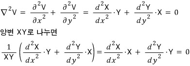
Editor’s note — 2 October 2026. The historical image correctly substitutes a product into Laplace’s equation but its final divided line multiplies by each factor where it should divide by that factor. After division, each factor’s second derivative is divided by that factor. Division is justified locally where both factors are nonzero; the undivided differential equations remain meaningful at zeros. The constant argument also requires the coordinates to vary independently.

For two terms with different variables to add up to zero, both terms must be constants!!

If you’ve got an objection to the claim that for (a function of x) + (a function of y) to give a constant, each function must itself be a constant, let’s hear it^^

I’ll call the constant k²…. (the reason I use a square is to make the calculation easier hehe, you’ll be able to catch why as we go further)

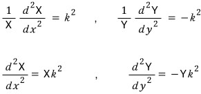
If you differentiate “something” twice,

and “something” comes out again, then that something must be of the form e-to-the-x (exponential) or a trig function (sine or cosine).

(The details are actually covered in differential equations ~original differential-equations post)

View the original linked-post preview thumbnail. Original linked-post preview thumbnail. This is the actual 220-by-220 thumbnail containing cropped Korean lettering. The original card’s title, excerpt, displayed domain and destination are preserved in English. Original preview destination.

Differential equations special post.

If you’re an undergraduate in engineering or the sciences, I’m going to post about “(linear) differential equations” which you’ll run into an absurd amount….

gdpresent.blog.me

Anyway, if I write out the general solution,

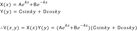
You make the general solution like this, and then plug in the boundary conditions one by one to find the coefficients A, B, C, D, k!!! hehehe fun, right!!

Editor’s note — 2 October 2026. These exponential and trigonometric expressions are the general solutions of the chosen one-coordinate differential equations. Their product is one separated solution, rather than the general solution of the full partial differential equation. The later mode sum supplies the freedom needed to match entrance data.

Let’s work through an example problem.

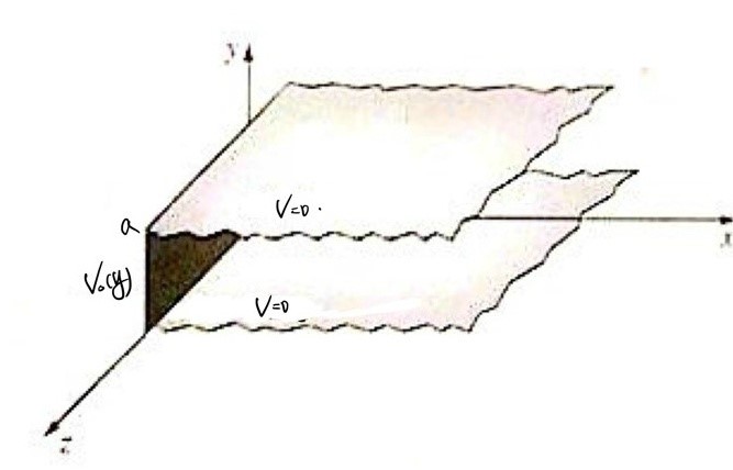
Let’s try using separation of variables under boundary conditions like these!!!

Since we did it in 2D, I brought a problem asking about V(x,y) in 2D too!

Let’s write out the boundary conditions first

1. V(x,0) = 0

2. V(x,a) = 0

3. V(∞,y) = 0

4. V(0,y) = V₀(y)

Editor’s note — 2 October 2026. The strip is charge-free, has constant permittivity and is independent of the third coordinate. The entrance function prescribes boundary values across an opening; a varying value does not describe one connected conductor in electrostatic equilibrium. Smooth data that vanish at the entrance endpoints give continuous agreement with the grounded side walls. Incompatible corner values instead require limits on the open boundary faces. The reviewed derivation also specifies boundedness and uniform transverse decay at infinity.

Now let’s plug them in one by one~~~~

From boundary condition 1, D=0

From boundary condition 2, Csin(ky) = 0 ☞ ∴k=nπ/a

From boundary condition 3, A=0

We can go up to here. As a result, we couldn’t determine the constants B and C.

Let’s go determine them!

First, if we write V with the constants we’ve determined so far applied,

View the historical strip-mode image. Historical strip-mode image. The Korean instruction says “B and C are undetermined coefficients, so let’s absorb and combine them into one constant.” Its exponent omits x, as explained in the adjacent editor’s note.

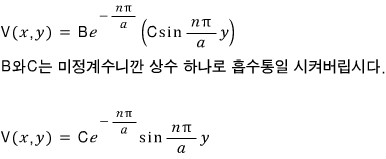
Editor’s note — 2 October 2026. The historical strip-mode image omits x from its decaying exponential. The exponent must depend on distance along the strip: minus the positive wave number times x. Without x, the displayed factor is constant along the strip and cannot supply the stated decay. Combining the two remaining amplitudes into one coefficient is valid.

Now you see why we took X’s general solution as an exponential and Y’s as a trig function, right?

If X had been a trig function, it wouldn’t have been able to make V=0 far away,

and if Y had been an exponential, it wouldn’t have been able to make V=0 at y=a and y=0.

(And there needs to be a condition n≠0 but I forgot to mention it..hehe)

And the reason I restricted n to positive values is that the sign of k flips back and forth, so I just decided on plus or minus either way.!!!

(It’s fine to take it as negative.)

Editor’s note — 2 October 2026. For a nonzero mode, the second wall condition is evaluated at y equal to a, giving a positive transverse wave number indexed by a positive integer. The zero mode is trivial under both grounded-wall conditions. Negative sine indices only repeat the same transverse shapes up to a sign; they do not permit changing a decaying exponential into a growing one. The signs of the separation constants are selected by these walls and longitudinal decay, rather than by convenience alone.

Anyway, we got V’s general solution like that.

How many general solutions does V have?? A ton…

The differential equation we dealt with is a linear one, so it also satisfies linear combination!!!(the sum of solutions is also a solution!)

Let’s do a linear combination and express the many solutions as one.

(For those who want the details, please check the linear algebra post^^ planned for June 2015^^)

View the historical strip-superposition image. Historical strip-superposition image. The Korean heading says “For reference: a linear combination,” followed by the weighted sum of modes. Its displayed strip series omits x from the exponential, as explained in the adjacent editor’s note.

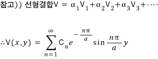
Editor’s note — 2 October 2026. This historical strip-series image also omits x from the exponential. A finite linear combination of harmonic modes is harmonic. For an infinite series, convergence and differentiation must be justified as well. The exponential factors in the corrected series control differentiated sums a positive distance from the entrance; boundary limits require their own conditions.

Now, if we plug boundary condition 4 — which didn’t get used earlier — into that general solution,

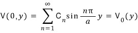
Now, how we’re going to cook this equation up is, we’ll use a purely mathematical technique called Fourier’s trick.

We’ll multiply both sides by sin(n’πy/a) and make a term that integrates from 0 to a

(Fourier’s trick is used a lot not just in electromagnetism, but also in thermal/statistical mechanics, quantum mechanics, etc.)

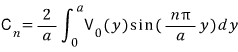
View the historical Fourier-coefficient step. Historical Fourier-coefficient step. The right-hand integration differential is missing; the adjacent editor’s note and complete scientific derivation supply it.

Editor’s note — 2 October 2026. The right-hand integral in the historical Fourier-step image is missing its integration differential. It is an integral over y from zero to a. With that differential supplied, sine orthogonality selects the matching coefficient and gives the normalization two divided by a used in the next formula.

Now on the left side, only when n=n’ does it give (a/2), and in all other cases it’s 0, so the left side becomes

0+0+0+0+0+Cₙ(a/2)+0+0+0+ ···················· so in the end

we get to determine the constant Cₙ.

<Functions whose inner product is zero are said to be orthogonal to each other. (When you view functions as vectors, the inner product is an integral.)>

Even if you don’t know what orthogonal means, you can just integrate and notice that everything except n=m is aaalll 0, so don’t worry about it.

(In linear algebra they cover the inner product of vectors other than spatial vectors.)

Let me solve one more with the Laplace equation in 3D.

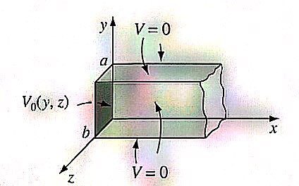
Let’s try with boundary conditions like these. Let’s write out the boundary conditions neatly first~

Just from a glance at the picture, you can catch that x should be in exponential form and y, z should be in sine form.

1. y=0 → V=0

2. y=a → V=0

3. z=0 → V=0

4. z=b → V=0

5. x→∞ → V=0

6. x=0 → V=V(y,z)

View the historical three-coordinate separation image. Historical three-coordinate separation image. Its derivative notation and middle-line axis assignments are inconsistent; the adjacent editor’s note distinguishes them from the intended exponential and sine factors shown later.

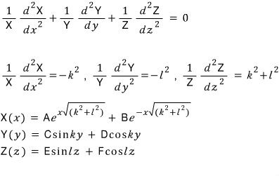
Editor’s note — 2 October 2026. The historical three-coordinate image has inconsistent derivative notation and assigns separation constants to the wrong axes in its middle line. The grounded y and z directions need negative squared wave numbers; the decaying x direction needs their positive sum. The exponential X factor and sine Y and Z factors shown afterward use this intended arrangement. Their product is one separated mode; the final pipe solution uses a double sum with two independently positive integer indices.

We’ve got the general solution for V(x,y,z).

Let’s plug in the boundary conditions one by one.

From boundary condition 1, D=0

From boundary condition 2, Csin(ky)=0, so k=nπ/a

From boundary condition 3, F=0

From boundary condition 4, Esin(lb)=0, so l=mπ/b

From boundary condition 5, A=0

View the original pipe-mode and double-sum image. Original pipe-mode and double-sum image. The Korean instruction says “Let’s absorb the undetermined coefficients B, C and E into C, and make a linear combination — a double sum — too!” The displayed pipe exponent and sine factors are mathematically correct. Its linked representation preserves the Korean instruction in English.

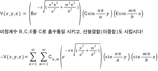
Now if we plug in the last boundary condition here!!!!!

Do Fourier’s trick for y separately, z separately, go go go go go

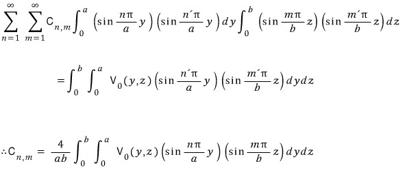
And just like that, we’ve found every single constant~~~~ If V₀(y,z) happens to be a function that doesn’t depend on y,z,

the next integration step is high-school level, so you can do it easy-peasy!

Editor’s note — 2 October 2026. A constant entrance value makes these coefficient integrals elementary, but a nonzero constant conflicts with the grounded walls where the entrance meets their edges or corners. The resulting formulas describe the harmonic interior and limits on the open faces, rather than a common continuous value at those junctions. The reviewed constant-entrance example makes this distinction explicit.

When I first did this I was like wow….. what the heck is this doing…?

but if you sit down caaalmly and follow it step by step, it’s really not that hard~

This was my midterm range~

and studying this way, I got the top score~ clap clap clap clap~~

I’ve gotta keep studying hard from here on! hehe

Reviewed scientific explanation

The following corrected English scientific edition and its dated correction are preserved in full; repeated images are referenced at their original-narrative locations.

The method of images solves some electrostatic boundary problems by replacing conductors with suitable imaginary charges. Separation of variables takes another route: it builds simple solutions that fit the geometry, then combines them to match the remaining boundary data.

This study note works through a grounded strip and a rectangular pipe. The useful habit is to ask which coordinate describes decay and which coordinates describe variation between grounded walls.

Refer to the original narrative image: Decorative cartoon sticker of a character thinking with a hand at its chin

From a product to ordinary differential equations

In a charge-free region with constant permittivity, the electrostatic potential satisfies Laplace’s equation. For a problem independent of the third coordinate, it reads

$$ \frac{\partial^2 V}{\partial x^2} +\frac{\partial^2 V}{\partial y^2}=0. $$

We first look for a nonzero separated mode of the form

$$ V(x,y)=X(x)Y(y). $$

Substitution gives

$$ X''(x)Y(y)+X(x)Y''(y)=0. $$

Primes denote ordinary derivatives of each factor with respect to its own coordinate. On a patch where both factors are nonzero, division by their product gives

$$ \frac{X''}{X}+\frac{Y''}{Y}=0. $$

The first ratio depends only on $x$ and the second only on $y$. Because these coordinates can vary independently, each ratio must be constant. For the grounded strip below, the useful choice is

$$ \frac{X''}{X}=k^2,\qquad \frac{Y''}{Y}=-k^2, $$

with $k>0$. Equivalently,

$$ X''=k^2X,\qquad Y''=-k^2Y. $$

Unlike the divided ratios, these ordinary differential equations remain meaningful where a factor vanishes. The retained source image records the same equations.

Refer to the original narrative image: Separated equations with positive k squared for X and negative k squared for Y

Their general one-coordinate solutions are

$$ \begin{aligned} X(x)&=Ae^{kx}+Be^{-kx},\\ Y(y)&=C\sin(ky)+D\cos(ky). \end{aligned} $$

The product $V=XY$ is one separated solution. It is not the general solution of the original partial differential equation.

Refer to the original narrative image: Exponential X factor, sine and cosine Y factor, and their product for the two-dimensional potential

A boundary potential usually needs a sum of modes. Separation succeeds here because the geometry supplies a suitable sine basis; it does not require the complete potential to be one product, or depend on a lucky guess.

A semi-infinite grounded strip

Take $a>0$. The strip extends along positive $x$, with $y$ strictly between $0$ and $a$. Its geometry and boundary data are independent of $z$, so we seek a $z$-independent potential.

Refer to the original narrative image: Grounded parallel walls at y equals zero and a, with entrance potential V zero of y at x equals zero and the strip extending along positive x

The two side walls are grounded:

$$ V(x,0)=V(x,a)=0. $$

At the open entrance we prescribe

$$ V(0,y)=g(y),\qquad g(y)=V_0(y). $$

Here $g$ specifies boundary values across the entrance. A varying $g$ does not describe a single connected conductor in electrostatic equilibrium, which would be an equipotential.

We seek a bounded harmonic potential that tends to zero uniformly across the strip as $x$ tends to infinity. First consider smooth entrance data that vanish at both endpoints, so the entrance and grounded walls agree at the corners.

Let the boundaries choose the modes

For a nontrivial product mode, the wall at $y=0$ gives $D=0$. The wall at $y=a$ then requires

$$ \sin(ka)=0,\qquad k=\frac{n\pi}{a}, $$

where $n$ is a positive integer. There is no nontrivial zero mode: a linear $Y$ vanishing at both endpoints is identically zero. A negative eigenvalue for $-Y''$ would give hyperbolic factors, and the same two zero boundary conditions again force the trivial solution. Negative integers only duplicate the sine modes up to a sign.

Decay along positive $x$ removes the growing exponential, so $A=0$. Absorb the product of the remaining amplitudes $BC$ into $C_n$. It is convenient to name the transverse and longitudinal factors:

$$ \begin{aligned} s_n(y)&=\sin\!\left(\frac{n\pi y}{a}\right),\\ r_n(x)&=e^{-n\pi x/a}. \end{aligned} $$

Then a mode and its superposition are

$$ \begin{aligned} V_n(x,y)&=C_n r_n(x)s_n(y),\\ V(x,y)&=\sum_{n=1}^{\infty}V_n(x,y). \end{aligned} $$

The $x$ in the exponential is essential: it makes the exponent dimensionless and produces the required decay. Each mode satisfies Laplace’s equation because its positive second derivative in $x$ cancels its negative second derivative in $y$.

Linearity guarantees that a finite sum is a solution. For an infinite sum, convergence and differentiation must also be justified. With the smooth data considered here, the exponential factors give uniform convergence of the series and its differentiated series whenever $x$ stays a positive distance from the entrance.

Find the Fourier coefficients

At $x=0$, every $r_n$ equals one. The remaining condition is the sine expansion

$$ g(y)=\sum_{n=1}^{\infty}C_n s_n(y). $$

Refer to the original narrative image: Entrance potential expressed as a Fourier sine series with coefficients C n

The sine functions are orthogonal on the transverse interval. For positive integers $n$ and $p$,

$$ \int_0^a s_n(y)s_p(y)\,dy =\frac{a}{2}\delta_{np}. $$

The Kronecker delta is one when the indices agree and zero otherwise. Multiply the entrance expansion by $s_p(y)$ and integrate over $y$. All other coefficients disappear, leaving

$$ \frac{a}{2}C_p=\int_0^a g(y)s_p(y)\,dy. $$

Rename the surviving index $n$ to obtain

$$ C_n=\frac{2}{a}\int_0^a g(y)s_n(y)\,dy. $$

This is the coefficient formula in the retained image, using $g=V_0$ and the definition of $s_n$ above.

Refer to the original narrative image: Fourier sine coefficient C n equals two over a times the integral of the entrance potential against its sine mode

The mode shapes already satisfy the differential equation, grounded walls and decay. Only the entrance data are needed to determine their amplitudes.

Boundary limits and uniqueness

The meaning of the entrance condition matters. For a piecewise smooth $g$, the sine series approaches $g$ at an interior continuity point and the average of its one-sided limits at an interior jump. Each sine term is zero at the endpoints. Thus nonzero endpoint data cannot also give a potential continuous at the corners where the entrance meets a grounded wall.

For smooth compatible data, the series gives a bounded harmonic solution with the stated continuous boundary values. It is unique among solutions with those values and uniform transverse decay. To see why, subtract two solutions and truncate the strip at $x=L$. Their difference is zero on the entrance and side walls. The maximum principle bounds its magnitude by its maximum on the far cross-section. Uniform decay makes that bound tend to zero as $L$ grows.

Discontinuous corner data require boundary limits on the open faces instead of continuity on the entire boundary. The elementary uniqueness argument just given assumes compatible continuous data; it should not silently be applied across a corner discontinuity.

A semi-infinite rectangular pipe

Now let $a,b>0$. The pipe extends along positive $x$, with $y$ between $0$ and $a$ and $z$ between $0$ and $b$. The four side walls are grounded. At $x=0$, the potential is prescribed on the open rectangular entrance.

Refer to the original narrative image: Rectangular pipe extending along x, with height a along y, width b along z, four grounded side walls and entrance potential V zero of y and z

The boundary conditions can be written as

$$ \begin{aligned} V(x,0,z)&=V(x,a,z)=0,\\ V(x,y,0)&=V(x,y,b)=0,\\ V(0,y,z)&=h(y,z). \end{aligned} $$

Here $h(y,z)=V_0(y,z)$. Again we require a bounded solution and decay to zero uniformly across the transverse rectangle as $x$ tends to infinity. Smooth entrance data compatible with the grounded edges provide a sufficient setting for the continuous boundary problem.

Separate the three coordinates

Start from $V(x,y,z)=X(x)Y(y)Z(z)$. The three-dimensional Laplace equation gives, on patches where the factors are nonzero,

$$ \frac{X''}{X}+\frac{Y''}{Y}+\frac{Z''}{Z}=0. $$

Each ratio is constant, and the constants sum to zero. The grounded transverse walls lead to the choice

$$ \begin{aligned} Y''&=-k^2Y,\\ Z''&=-l^2Z,\\ X''&=(k^2+l^2)X. \end{aligned} $$

Thus $y$ and $z$ carry the sine modes, while $x$ carries the exponential decay. With

$$ \kappa=\sqrt{k^2+l^2}>0, $$

the separate factors are

$$ \begin{aligned} X(x)&=Ae^{\kappa x}+Be^{-\kappa x},\\ Y(y)&=C\sin(ky)+D\cos(ky),\\ Z(z)&=E\sin(lz)+F\cos(lz). \end{aligned} $$

Their product $V=XYZ$ is the expression in the retained source image.

Refer to the original narrative image: Product of a longitudinal exponential factor and two transverse sine and cosine factors for the rectangular pipe

The walls at $y=0$ and $z=0$ set $D=F=0$. The opposite walls quantize the transverse wave numbers:

$$ k=\frac{n\pi}{a},\qquad l=\frac{m\pi}{b}. $$

The integers $n$ and $m$ are independently positive. Decay sets $A=0$, and the amplitude $BCE$ becomes one coefficient $C_{nm}$.

Retain $s_n(y)$ from the strip and define

$$ \begin{aligned} t_m(z)&=\sin\!\left(\frac{m\pi z}{b}\right),\\ \kappa_{nm}&=\pi\sqrt{\frac{n^2}{a^2}+\frac{m^2}{b^2}},\\ S_{nm}(y,z)&=s_n(y)t_m(z). \end{aligned} $$

At a point $(x,y,z)$, write the decaying mode value as $U_{nm}$. The modes and their sum are

$$ \begin{aligned} U_{nm}&=C_{nm}e^{-\kappa_{nm}x}S_{nm}(y,z),\\ V(x,y,z)&=\sum_{n=1}^{\infty}\sum_{m=1}^{\infty}U_{nm}. \end{aligned} $$

The transverse second derivatives contribute negative squared wave numbers. Their sum cancels the positive longitudinal contribution $\kappa_{nm}^2$, so each mode is harmonic. The sine factors vanish on all four sides, and the exponential decays along the pipe.

Apply orthogonality in both directions

At the entrance the double series becomes

$$ h(y,z)=\sum_{n=1}^{\infty}\sum_{m=1}^{\infty}C_{nm}S_{nm}(y,z). $$

Refer to the original narrative image: Entrance potential expanded in a double sine series, with independent y and z mode indices

The $y$ integral supplies the factor $a/2$ as before. In the other direction,

$$ \int_0^b t_m(z)t_q(z)\,dz =\frac{b}{2}\delta_{mq}. $$

Multiply the entrance expansion by $S_{pq}(y,z)$ and integrate over the rectangle. Orthogonality in both coordinates selects $C_{pq}$. To keep the integral readable, define its integrand and value separately:

$$ \begin{aligned} F_{pq}(y,z)&=h(y,z)S_{pq}(y,z),\\ I_{pq}&=\int_0^b\!\int_0^a F_{pq}(y,z)\,dy\,dz. \end{aligned} $$

The inner integral is over $y$ from zero to $a$; the outer one is over $z$ from zero to $b$. The selected coefficient therefore obeys

$$ \frac{ab}{4}C_{pq}=I_{pq}. $$

Renaming the two surviving indices gives the result

$$ C_{nm}=\frac{4}{ab}I_{nm}. $$

Together with the definitions of $F_{nm}$ and $S_{nm}$, this says to integrate $h(y,z)$ against both sine factors and multiply by $4/(ab)$. The retained source image shows the expanded calculation with primed indices.

Refer to the original narrative image: Double sine orthogonality calculation and coefficient normalized by four over a b, integrating over y first and z second

For smooth compatible data, this expansion gives the prescribed boundary limits and a harmonic interior solution. Exponential decay again controls differentiated sums away from the entrance. We do not need a claim that an arbitrary double Fourier series converges pointwise everywhere. The same truncated-domain maximum-principle argument establishes uniqueness for the continuous compatible problem with uniform decay.

Check the result with a constant entrance potential

Suppose the strip entrance has the constant value $g(y)=V_c$. Direct integration gives

$$ C_n=\frac{2V_c}{n\pi}\bigl[1-(-1)^n\bigr]. $$

Thus even coefficients vanish, while an odd index gives $C_n=4V_c/(n\pi)$.

For the pipe with $h(y,z)=V_c$, the two integrals separate. Let

$$ P_j=1-(-1)^j. $$

Then

$$ C_{nm}=\frac{4V_c}{nm\pi^2}P_nP_m. $$

If either index is even, the coefficient is zero. When both are odd,

$$ C_{nm}=\frac{16V_c}{nm\pi^2}. $$

A nonzero constant entrance value conflicts with the grounded walls at the entrance corners or edges. These formulas describe the bounded harmonic interior solution and its limits on the open entrance and open side walls; they do not assign a common continuous value where those faces meet.

This is a useful check on the factors of two, the two independent indices and the direction of decay. More generally, inspect a proposed mode by differentiating it, evaluating it on each grounded wall and checking its behavior far down the strip or pipe. The final entrance expansion then determines how much of each mode is needed.

Refer to the original narrative image: Decorative cartoon sticker of a smiling character holding up both hands

Editorial correction and sources

Editorial correction — 2026-09-12. This is a corrected English edition of the original study note, not an unchanged literal translation. Three misassigned local images were first restored from the original live source. The obsolete external-link preview was then removed from display. Seven historical image occurrences were retired from display; all original and restored files remain preserved.

The readable mathematics corrects the divided Laplace expression, restores missing $x$ factors in exponential decays, supplies a missing integration differential and corrects the three-dimensional derivative notation and axis assignments. Korean explanatory image text is replaced by English prose and native mathematics. The original pipe-series exponent and sine factors were already correct. Eleven source images remain displayed unchanged, with English descriptions and readable mathematical equivalents for every retained equation image.

The derivation was cross-checked against Richard Fitzpatrick’s Separation of variables and the University of Texas at Austin course notes Separation of Variables Method. The first reference uses a strip width of $\pi$; this note uses $a$. In the course notes’ pipe example, the decay coordinate is $z$; here it is $x$, with transverse coordinates $y,z$. The first reference’s equations 777 and 797 contain derivative and sine-coordinate typos; the formulas here follow direct differentiation and the stated boundaries.