Electric Displacement

The original learning narrative, in full

The following preserves the original study-note sequence. Notes dated 2026-10-02 clarify its developing intuition; the complete corrected scientific explanation follows in the appendix.

Original Korean learning note

What we have learned so far while studying polarization density is this:

We could use polarization—the polarization density—to calculate the charge density bound inside a dielectric and the charge density on its outer surface.

Historical source image 1: Bound surface charge density equals P dotted with the outward normal; bound volume charge density equals minus divergence of P.

\[ \sigma_b=\mathbf P\cdot\hat{\mathbf n},\qquad\rho_b=-\nabla\cdot\mathbf P. \]

Like this, y’know.

The electric field created again when the medium becomes polarized is due to that!!! That bound charge density right there!!! (We caught the culprit.)

Editorial note (2026-10-02): The polarization field determines bound charge, whose electric field contributes to the total field. A linear separation of source contributions can be useful, but it must be distinguished from the definition of D.

Now then, our interest (for now) is ‘inside the dielectric.’

Some other electric field polarizes the material, and then another electric field is created there, right?

The total electric field “inside this dielectric” = all kinds of external electric fields + the electric field formed inside the dielectric because of polarization.

Let us divide it into these two kinds.

Historical source image 2: Historical decomposition: total E equals external E plus polarization E. The Korean subscripts mean total, external, and polarization.

\[ E_{\mathrm{total}}=E_{\mathrm{external}}+E_{\mathrm{polarization}}. \]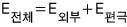

Here, using \(\nabla E=\rho/\varepsilon\) and \(\rho_b=-\nabla P\), let us change the expression into one involving rho.

Editorial note (2026-10-02): The prose shorthand omits the dot indicating divergence and the vacuum-permittivity subscript. The scalar relations are divergence of E equals total charge density divided by epsilon-zero, and bound volume charge density equals minus divergence of P. Source image 3 also omits the divergence dot in its second line; its gradient of a vector sum is not the intended scalar divergence. The complete corrected native derivation is preserved in the appendix.

Historical source image 3: Historical rearrangement: epsilon-zero times divergence of E equals external rho minus divergence of P; the second line writes external rho as gradient of the sum epsilon-zero E plus P, with no divergence dot.

\[ \begin{aligned}\varepsilon_0\nabla\cdot\mathbf E&=\rho_{\mathrm{external}}-\nabla\cdot\mathbf P,\\\rho_{\mathrm{external}}&=\nabla(\varepsilon_0\mathbf E+\mathbf P).\end{aligned} \]

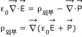
<Do not forget. E is the total! electric field inside the dielectric~>

From that expression, I will define a new vector D.

Historical source image 4: Epsilon-zero times E plus P equals D.

\[ \varepsilon_0\mathbf E+\mathbf P=\mathbf D. \]

D: the replacement electric field (Electric displacement). That is, that is, that is, that is, that is, that is…

Editorial note (2026-10-02): “Replacement electric field” is the author’s learning phrase. The conventional English name is electric displacement field; D has units of charge per area rather than electric-field units.

Historical source image 5: Historical free-charge laws: external rho equals divergence of D; enclosed free Q equals the integral of D followed by the vector area element, with no explicit dot.

\[ \rho_{\mathrm{external}}=\nabla\cdot\mathbf D,\qquad Q_{\mathrm{in(free)}}=\oint\mathbf D\,d\mathbf a. \]

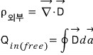
Editorial note (2026-10-02): Source image 5 writes the integral of D followed by a vector area element without an explicit dot. The free-charge flux law requires the scalar dot product D·d(vector a). The label “external” is translated literally in the historical expressions; the precise source quantity is enclosed free charge, not merely charge outside the dielectric.

It looks like something we have seen somewhere before, right? Haha.

Historical source image 6: Gauss’s law: divergence of E equals rho divided by epsilon-zero; the E flux equals enclosed Q divided by epsilon-zero.

\[ \nabla\cdot\mathbf E=\frac{\rho}{\varepsilon_0},\qquad\oint\mathbf E\cdot d\mathbf a=\frac{Q_{\mathrm{in}}}{\varepsilon_0}. \]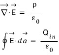

It reminds me of this.

When there is no dielectric, D and E would be the same, right?

Editorial note (2026-10-02): In vacuum P is zero, so D = epsilon-zero times E. D and E are not equal in SI units. The later outside-dielectric formula in this same original note states the correct scaling.

But when there is a dielectric, let us use D—that is what I mean.

The D vector is! “All kinds of electric fields except the polarization effect”!

Editorial note (2026-10-02): D is an auxiliary field defined by epsilon-zero times the total E plus P. It is not generally an electric-field component with polarization subtracted; its divergence law alone does not determine D without symmetry and boundary conditions.

Let us compare it with E while solving a problem.

Historical source image 7: A straight wire uniformly carrying line charge lambda is wrapped in insulating rubber of radius a. Find D. The drawing marks the radius a and the line charge lambda.

\[ \lambda\quad\text{(uniform line charge)},\qquad a\quad\text{(rubber radius)};\qquad\text{find }\mathbf D. \]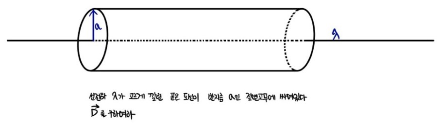

Editorial note (2026-10-02): The setup image says a straight uniformly charged wire is wrapped in insulating rubber of radius a. The cylindrical Gaussian derivation assumes an infinitely long line or negligible end effects and cylindrical symmetry; these assumptions are stated explicitly in the scientific appendix.

First, this is the problem. Let us pretend the insulating rubber is not wrapped around it and find the electric field due to the wire.

Using Gauss’s law,

Historical source image 8: Vacuum cylindrical Gaussian calculation: E times two pi s L equals enclosed Q divided by epsilon-zero, equal to lambda L divided by epsilon-zero; vector E equals lambda over two pi epsilon-zero s times s-hat.

\[ \begin{aligned}E(2\pi sL)&=\frac{Q_{\mathrm{in}}}{\varepsilon_0}=\frac{\lambda L}{\varepsilon_0},\\\mathbf E&=\frac{\lambda}{\varepsilon_0}\frac{1}{2\pi s}\hat{\mathbf s}.\end{aligned} \]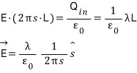

Now, let us bring the insulating rubber back and combine them!

Then do not forget that there is also a polarization effect!! If polarization has an effect, well~ it is difficult to calculate, so…

Let us use the replacement electric field. (We have no information about the total electric field or the polarization density; we only have the external line charge density lambda…)

Since D considers the inside of the dielectric, it would be a greater than s, right?

Editorial note (2026-10-02): The inside calculation uses zero less than s less than a, but D is defined outside the dielectric too. Under this cylindrical symmetry its radial free-charge flux result holds on either side of the interface.

Historical source image 9: Cylindrical displacement calculation: D times two pi s L equals enclosed free Q, equal to lambda L; vector D equals lambda over two pi s times s-hat.

\[ \begin{aligned}D(2\pi sL)&=Q_{\mathrm{in(free)}}=\lambda L,\\\mathbf D&=\frac{\lambda}{2\pi s}\hat{\mathbf s}.\end{aligned} \]

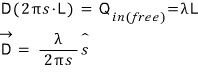
Now, have a look. Because of the line charge density you see there, the electric field a distance s away in the vibrating state is like that,

Editorial note (2026-10-02): The original says “vibrating state” here; the surrounding vacuum calculation makes “vacuum state” the likely intended wording. The historical wording is retained and this probable typo is identified explicitly.

and if it is not in vacuum, the replacement electric field due to the line charge density a distance s away is like that.

I think we can find the reason they differ by a factor of one over epsilon-zero by looking at the “dielectric.”

Editorial note (2026-10-02): The factor one over epsilon-zero compares the differently dimensioned vacuum electric field and displacement field in this symmetric example. It is not the physical reduction factor for the electric field due to the dielectric. For a homogeneous linear dielectric, the inside electric field is its vacuum value times epsilon-zero divided by the material permittivity.

Bound charge density spreads all over the dielectric, so there is a little change,

and now we can express all those kinds of external electric fields using the total electric field and polarization, right?

I do not know whether you are getting a feel for it yet.

What about outside the dielectric? Outside the dielectric, P is zero, right???

Since D = epsilon-zero times E, the electric field outside the dielectric is simply E = D divided by epsilon-zero.

It may look very~ easy, but without using D, we would have to find the total electric field by considering the effects of all kinds of external charge densities and the surface charge densities created by polarization.

Editorial note (2026-10-02): Bound volume charge may also contribute. In a prescribed or spatially varying polarization distribution one must include both bound volume and surface charges when using the E law directly.

So in this case too, using D is convenient.

Historical source image 11: There is a dielectric spherical shell. Inner radius: a. Outer radius: b. Its polarization density exists in the form P(r) = k over r times r-hat.

\[ a\quad\text{(inner radius)},\qquad b\quad\text{(outer radius)},\qquad\mathbf P(r)=\frac{k}{r}\hat{\mathbf r}. \]

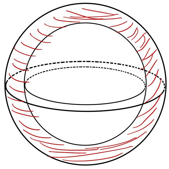
For this problem, let us find the electric field once using E,

and solve the problem once using D.

First, let us solve it by considering the electric fields one by one.

Historical source image 12: For r less than a, the E flux and enclosed Q vanish, so the source concludes vector E equals zero.

\[ r\lt a:\qquad\oint\mathbf E\cdot d\mathbf a=0\quad(\because Q_{\mathrm{in}}=0),\qquad\therefore\mathbf E=0. \]

Historical source image 13: For r greater than b, the E flux and enclosed Q vanish, so the source concludes vector E equals zero.

\[ r\gt b:\qquad\oint\mathbf E\cdot d\mathbf a=0\quad(\because Q_{\mathrm{in}}=0),\qquad\therefore\mathbf E=0. \]

Historical source image 14: Historical shell calculation for a less than r less than b. The Korean annotation asks: “The bound charge enclosed by the Gaussian surface is the inner surface and the volume bound charge between a and r, right?!” The inner surface charge density is minus k over a; the bound volume charge density is minus k over r squared. Their enclosed charges sum to minus four pi k a minus four pi k(r−a); the next printed equality is minus four pi r, missing k. The final electric field contains k and equals minus k over epsilon-zero r times r-hat.

\[ \begin{aligned}a\lt r\lt b:\quad\oint\mathbf E\cdot d\mathbf a&=\frac{1}{\varepsilon_0}\int\rho\,d\tau,\\\sigma_{\mathrm{inner\,bound}}&=\mathbf P(a)(-\hat{\mathbf r})=-\frac{k}{a}|\hat{\mathbf r}|=-\frac{k}{a},\\\rho_{\mathrm{bound}}&=-\nabla\cdot\mathbf P=-\frac{1}{r^2}\frac{\partial}{\partial r}\left[r^2\frac{k}{r}\right]=-\frac{k}{r^2},\\Q_{\mathrm{in}}&=\oint_S\sigma_{\mathrm{inner\,bound}}\,da+\int_V\rho_{\mathrm{bound}}\,d\tau\\&=-\frac{k}{a}(4\pi a^2)-\int_a^r\frac{k}{r^2}r^2\sin\theta\,dr\,d\theta\,d\varphi\\&=-4\pi ka-4\pi k(r-a)=-4\pi r,\\\mathbf E&=\frac{\hat{\mathbf r}}{4\pi r^2\varepsilon_0}Q_{\mathrm{in}}=-\frac{1}{\varepsilon_0}\frac{k}{r}\hat{\mathbf r}.\end{aligned} \]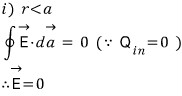

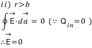
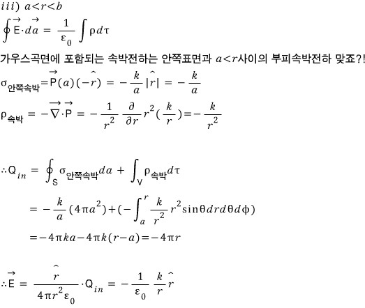
Editorial note (2026-10-02): The historical inner-boundary expression omits an explicit dot in P(a)(−r-hat). Its final intermediate enclosed-charge result also drops k, writing minus four pi r after two terms proportional to k; the correct value is minus four pi k r, consistent with the source’s final E. At the outer region, zero field follows from cancellation of all inner-surface, volume, and outer-surface bound charges plus spherical symmetry. The appendix preserves the full corrected calculation.

Now let us find E using the D vector.

Are there any other kinds of external electric fields here???? In other words, there are no other kinds of charge density besides polarization, right??

Historical source image 15: Historical D solution: zero enclosed free charge gives zero D flux, then D = 0 and E = −P divided by epsilon-zero in a less than r less than b. The Korean annotations say: “Done right away! Heh. When r is not between a and b, it is zero, so E is zero too. You understand, right?!?!?! Done~.”

\[ \begin{aligned}\oint\mathbf D\cdot d\mathbf a&=Q_{\mathrm{in(free)}}=0,\\\therefore\quad\mathbf D&=0,\\\varepsilon_0\mathbf E+\mathbf P&=0,\\\therefore\quad\mathbf E(r)&=-\frac{\mathbf P(r)}{\varepsilon_0}=-\frac{1}{\varepsilon_0}\frac{k}{r}\hat{\mathbf r}\qquad(a\lt r\lt b).\end{aligned} \]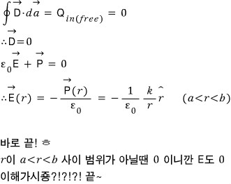

Editorial note (2026-10-02): Zero enclosed free-charge flux implies D = 0 here only after spherical symmetry and regular boundary behavior are used. Zero divergence or zero total flux alone would not imply that an arbitrary vector field vanishes. Outside the shell the zero quantity used in E = −P/epsilon-zero is P; the complete piecewise E and D arguments are retained in the appendix.

Scientific appendix: the complete corrected explanation

In the previous post on bound charge, we found that a polarization field \(\mathbf P\) produces

\[ \sigma_b=\mathbf P\cdot\hat{\mathbf n}, \qquad \rho_b=-\nabla\cdot\mathbf P. \]

Here \(\sigma_b\) is the bound surface charge on a dielectric-vacuum boundary, with \(\hat{\mathbf n}\) pointing outward from the dielectric, and \(\rho_b\) is the bound volume charge in a smooth polarized region. These are charges associated with the material’s polarization. They are distinct from free charge: charge placed on a conductor, supplied by an external circuit, or otherwise not represented by \(\mathbf P\).

The distinction suggests a useful auxiliary field. Instead of placing free and bound charge together on the right-hand side of Gauss’s law, we can absorb the bound-charge contribution into a new field, \(\mathbf D\).

Deriving the electric displacement field

The total charge density is

\[ \rho_{\mathrm{tot}}=\rho_f+\rho_b, \]

where \(\rho_f\) is free charge density. The differential form of Gauss’s law is therefore

\[ \nabla\cdot\mathbf E =\frac{\rho_f+\rho_b}{\varepsilon_0}. \]

Substitute \(\rho_b=-\nabla\cdot\mathbf P\):

\[ \begin{aligned} \varepsilon_0\nabla\cdot\mathbf E &=\rho_f-\nabla\cdot\mathbf P,\\ \nabla\cdot\left(\varepsilon_0\mathbf E+\mathbf P\right) &=\rho_f. \end{aligned} \]

This motivates the definition

\[ \boxed{\mathbf D\equiv\varepsilon_0\mathbf E+\mathbf P}. \]

Its Maxwell equation is

\[ \boxed{\nabla\cdot\mathbf D=\rho_f}. \]

Integrating over a volume \(V\) and applying the divergence theorem gives the integral form:

\[ \boxed{ \oint_{\partial V}\mathbf D\cdot d\mathbf a =Q_{f,\mathrm{enc}} }. \]

Only the enclosed free charge appears on the right. For comparison,

\[ \oint_{\partial V}\mathbf E\cdot d\mathbf a =\frac{Q_{f,\mathrm{enc}}+Q_{b,\mathrm{enc}}}{\varepsilon_0}. \]

Across an interface, a pillbox version of the \(\mathbf D\) law gives

\[ \hat{\mathbf n}\cdot(\mathbf D_2-\mathbf D_1)=\sigma_f, \]

where \(\sigma_f\) is free surface charge and \(\hat{\mathbf n}\) points from region 1 to region 2.

What \(\mathbf D\) does—and does not—mean

It is tempting to call \(\mathbf D\) “the electric field with polarization removed.” That is not generally correct. The quantities even have different SI units:

\[ [\mathbf E]=\mathrm{V/m}, \qquad [\mathbf D]=[\mathbf P]=\mathrm{C/m^2}. \]

The definition \(\mathbf D=\varepsilon_0\mathbf E+\mathbf P\) is a reorganization of Gauss’s law. It lets us track free charge separately from the bound charge already encoded by \(\mathbf P\). It does not mean that \(\mathbf D\) is the sum of “all electric fields except the polarization field,” and \(\nabla\cdot\mathbf D=\rho_f\) does not by itself determine \(\mathbf D\). We still need symmetry, boundary conditions, or other Maxwell equations.

The definition and the free-charge Maxwell equation are material-independent. A constitutive relation is additional information about a particular material. For a homogeneous, isotropic, linear dielectric,

\[ \mathbf P=\varepsilon_0\chi_e\mathbf E, \qquad \mathbf D=\varepsilon\mathbf E, \qquad \varepsilon=\varepsilon_0(1+\chi_e). \]

The shortcut \(\mathbf D=\varepsilon\mathbf E\) is not universal. In an anisotropic medium, \(\varepsilon\) may be a tensor; in a nonlinear or history-dependent material, \(\mathbf D\) need not be proportional to \(\mathbf E\) at all. In vacuum, \(\mathbf P=0\), so \(\mathbf D=\varepsilon_0\mathbf E\)—not \(\mathbf D=\mathbf E\).

Example 1: a line charge inside a dielectric cylinder

Consider an infinitely long free line charge of density \(\lambda\) on the axis of a cylindrical dielectric of radius \(a\). Assume cylindrical symmetry, a homogeneous linear dielectric of permittivity \(\varepsilon\) for \(0\lt s\lt a\), vacuum for \(s\gt a\), and no free charge on the interface \(s=a\). The ideal line \(s=0\) is singular, so the following fields apply for \(s\gt 0\).

First imagine the dielectric absent. A coaxial Gaussian cylinder of radius \(s\) and length \(L\) gives

\[ E(2\pi sL)=\frac{\lambda L}{\varepsilon_0}, \qquad \mathbf E_{\mathrm{vac}}(s) =\frac{\lambda}{2\pi\varepsilon_0s}\,\hat{\mathbf s}. \]

Now restore the dielectric. Applying the \(\mathbf D\) flux law to the same Gaussian cylinder gives

\[ D(2\pi sL)=\lambda L, \qquad \boxed{ \mathbf D(s)=\frac{\lambda}{2\pi s}\,\hat{\mathbf s} } \quad(s\gt 0). \]

This result holds on both sides of \(s=a\) because every such Gaussian cylinder encloses the same free line charge and the assumed symmetry fixes the direction and magnitude. The normal component of \(\mathbf D\) is continuous at \(s=a\) because there is no free surface charge there.

The electric field follows only after we use the constitutive relation in each region:

\[ \mathbf E(s)= \begin{cases} \displaystyle \frac{\lambda}{2\pi\varepsilon s}\,\hat{\mathbf s}, & 0\lt s\lt a,\\[8pt] \displaystyle \frac{\lambda}{2\pi\varepsilon_0 s}\,\hat{\mathbf s}, & s\gt a. \end{cases} \]

Thus the dielectric reduces \(|\mathbf E|\) relative to its vacuum value by the factor \(\varepsilon_0/\varepsilon\) inside the material. The displacement field is not restricted to the dielectric: outside, it remains \(\mathbf D=\varepsilon_0\mathbf E\).

Example 2: a radially polarized spherical shell

Now consider a dielectric occupying the spherical shell \(a\lt r\lt b\), with prescribed polarization

\[ \mathbf P(r)=\frac{k}{r}\,\hat{\mathbf r} \qquad(a\lt r\lt b), \]

and \(\mathbf P=0\) elsewhere. Assume electrostatics, spherical symmetry, and no free charge anywhere.

Diagram already shown above: Hand-drawn spherical shell with concentric inner and outer boundaries; red hatching marks the dielectric material

Solution from the bound charges

In the shell,

\[ \rho_b =-\nabla\cdot\mathbf P =-\frac{1}{r^2}\frac{d}{dr}\!\left(r^2\frac{k}{r}\right) =-\frac{k}{r^2}. \]

At the inner boundary, the outward normal of the dielectric is \(-\hat{\mathbf r}\); at the outer boundary, it is \(+\hat{\mathbf r}\). Therefore

\[ \sigma_b(a)=-\frac{k}{a}, \qquad \sigma_b(b)=\frac{k}{b}. \]

For \(r\lt a\), a centered Gaussian sphere encloses no charge, so spherical symmetry gives \(\mathbf E=0\). For \(a\lt r\lt b\), the enclosed bound charge is

\[ \begin{aligned} Q_{b,\mathrm{enc}}(r) &=4\pi a^2\sigma_b(a) +\int_a^r\rho_b(r')\,4\pi r'^2\,dr'\\ &=-4\pi ka-4\pi k(r-a)\\ &=-4\pi kr. \end{aligned} \]

Gauss’s law then gives

\[ \mathbf E(r) =\frac{Q_{b,\mathrm{enc}}(r)}{4\pi\varepsilon_0r^2}\,\hat{\mathbf r} =-\frac{k}{\varepsilon_0r}\,\hat{\mathbf r}, \qquad a\lt r\lt b. \]

For \(r\gt b\), the inner surface charge, volume charge, and outer surface charge sum to zero:

\[ -4\pi ka-4\pi k(b-a)+4\pi kb=0, \]

so \(\mathbf E=0\) there as well. Altogether,

\[ \mathbf E(r)= \begin{cases} \mathbf 0, & r\lt a,\\[3pt] \displaystyle -\frac{k}{\varepsilon_0r}\,\hat{\mathbf r}, & a\lt r\lt b,\\[8pt] \mathbf 0, & r\gt b. \end{cases} \]

Solution from \(\mathbf D\)

Because there is no free charge,

\[ \oint\mathbf D\cdot d\mathbf a=0. \]

For a centered spherical Gaussian surface, symmetry requires \(\mathbf D=D(r)\hat{\mathbf r}\), so

\[ 4\pi r^2D(r)=0 \quad\Longrightarrow\quad \mathbf D=0 \]

in each region. The conclusion uses spherical symmetry and the regular boundary behavior; zero divergence alone would not be enough. Inside the polarized shell,

\[ \mathbf 0=\varepsilon_0\mathbf E+\mathbf P \quad\Longrightarrow\quad \mathbf E(r)=-\frac{\mathbf P(r)}{\varepsilon_0} =-\frac{k}{\varepsilon_0r}\,\hat{\mathbf r}. \]

Outside the shell, \(\mathbf P=0\), so \(\mathbf D=\varepsilon_0\mathbf E=0\). This agrees with the explicit bound-charge calculation.

The advantage of \(\mathbf D\) is now precise: its flux law isolates free charge. When symmetry makes that law solvable, it can spare us from summing the bound charges one by one. The material response is still present—it enters through \(\mathbf P\) or through an appropriate constitutive relation when we recover \(\mathbf E\).