Laplace's Equation

These are my original study notes, translated with their informal voice restored. Dated editorial clarifications are separate from the historical explanation, including its mistakes. The equations and previously reviewed image edits from the earlier English edition are retained.

Finally chapter 2 is done and chapter 3, the “potential” part, has started.

From here on, the content goes beyond the high-school physics level

Finally, after paying tuition, I’m getting to learn at university what I hadn’t learned until now!!

Let’s work hard so the money isn’t wasted

Of course I’m not studying because of the money hehehehe heheh

From charges to potential

In the previous chapter, almost at the very beginning,

we learned this content

You haven’t seen this equation before, right? Before, instead of going by charge density, we figured out the electric field using the qn charges at each position, right???

I went “well if those q’s are distributed continuously, it’d be an integral~” and didn’t write down the equation… but I’ll write it down now.

r is the distance from the origin

and eta is the distance from r,

so clearly they’re different things! which is why I notated them differently ha~~

So now, we can compute V with charge density too.

Now, even though this equation is logical;; actually calculating the integral with those numerical values isn’t easy

No, just doing an integral itself is hard!!!!!

Rather than integrating, differentiating is easier, isn’t it?

That’s why ~ earlier we learned all the differential forms ~

Editorial clarification (2 October 2026): From a charge distribution to the potential.

The historical text calls r the distance from the origin and eta the distance from r. The following retained equations make the source point, observation point, and their displacement explicit; that clarification is editorial, rather than a claim that the original notation already distinguished them correctly.

For a continuous charge distribution, Coulomb’s sum becomes an integral. Keep the observation point $\mathbf r$ distinct from the source point $\mathbf r'$. The displacement from source to observer is $\mathbf s$, its length is $s$, and its unit vector is $\hat{\mathbf s}$:

$$ \mathbf s=\mathbf r-\mathbf r',\qquad s=|\mathbf s|. $$$$ \hat{\mathbf s}=\frac{\mathbf s}{s},\qquad k=\frac{1}{4\pi\epsilon_0}. $$

Here $\epsilon_0$ is the vacuum permittivity. In free space, a localized charge distribution with convergent integrals gives the vector electric field

$$ \mathbf E(\mathbf r)=k\int_{\mathbb R^3}\rho(\mathbf r')\frac{\mathbf s}{s^3}\,d^3r'. $$

With the reference potential chosen to approach zero at infinity, the scalar potential is

$$ V(\mathbf r)=k\int_{\mathbb R^3}\frac{\rho(\mathbf r')}{s}\,d^3r'. $$

The field and potential have different kernels. Both integrals run over source coordinates while the observation point stays fixed. MIT’s treatment of charge distributions develops this distinction.

These free-space expressions require the complete charge distribution, including any induced charges. When conductor potentials are given but their surface charges are unknown, a boundary-value formulation can be more useful. Solving its differential equation may still be difficult; boundary conditions remain essential.

Poisson’s equation and Laplace’s equation

Integration is hard, so… what we had was

The front equation was the one we derived by proving electric force is conservative (curlE = 0),

realizing aha~ energy doesn’t depend on path~, and then computing the potential,

and the back equation was the one we derived while studying Gauss’s theorem!!!

I’ll substitute the front equation into the back one.

In conclusion, the equation colored in red is what gets derived, and that equation is called “Poisson’s equation.”

In the special case when the charge density is 0,

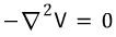
kind of obvious.

This obvious equation is called Laplace’s equation.

We’re now going to study Laplace’s equation.

(As you follow along~ you might wonder “what am I doing right now?” and be like what is this…

just keep following along, I also found as I kept going, at some moment~ I’d realize oh, this is what I was doing~ that’s how it went for me)

Like this

I’ll write down Laplace’s equation again and keep going with the explanation

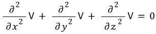
Everyone, what a “harmonic function” is~ a harmonic function is a function that satisfies the Laplace differential equation.

So the V potential function above also satisfies Laplace’s equation, so it’s a harmonic function.

We’ll briefly look into this harmonic function

Editorial clarification (2 October 2026): Poisson’s equation and the charge-free case.

The historical first field–potential image omitted the minus sign; its substitution image omitted the divergence dot. Those source images remain preserved in the evidence. The already accepted English equations below state the corrected relations. The original red Poisson result and negative-Laplacian-equals-zero image were already correct.

In electrostatics in vacuum, the potential relation and Gauss’s law are

$$ \mathbf E=-\nabla V, $$$$ \nabla\cdot\mathbf E=\frac{\rho}{\epsilon_0}. $$

The minus sign makes the field point toward decreasing potential. Electrostatic work between fixed endpoints is path-independent, and potential difference is minus the field’s line integral. The local condition is $\nabla\times\mathbf E=0$; deriving a global scalar potential from that condition alone also requires suitable topology, such as a simply connected region.

Substitute the negative gradient into Gauss’s law:

$$ \nabla\cdot(-\nabla V)=-\nabla^2V=\frac{\rho}{\epsilon_0}. $$

Equivalently, Poisson’s equation is

$$ \nabla^2V=-\frac{\rho}{\epsilon_0}. $$

These signs agree with the University of Texas derivation. In an open region where the charge density vanishes, the right-hand side is zero. The original charge-free equation shown earlier correctly retains a minus sign on the left.

Multiplying by minus one gives the usual form, $\nabla^2V=0$: Laplace’s equation. A twice continuously differentiable function satisfying it is called harmonic. This description applies inside the charge-free region, excluding charge singularities and charged surfaces. It does not require the potential or field to vanish.

The retained three-dimensional Cartesian equation is shown above.

One dimension

“1D Laplace equation” — 1D is very obvious but in 2D and 3D you can get dazed, so you’ve gotta watch carefully!!!

Since it’s 1D, V has 1 variable, and

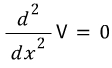
this is it, right? (Since there’s no need for partial derivatives, I just went with ordinary derivatives)

The solution for V(x) can be found real~ly easily

V(x)=ax + b

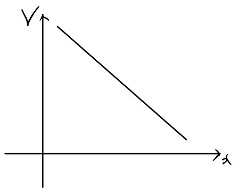
Let’s say it looks like this (just for the sake of explanation, I picked it arbitrarily~)

If I try to explain in my own way why the second derivative of V being 0 means something,

when x changes by this~~~much, V changes by ΔV.

Then when x changes by this~~~much again, V will also change by some ΔV, whatever that amount is hehe

The difference between these two ΔV’s being 0 is what “second derivative is 0” means

((Really simply, from a mechanics viewpoint, it means the change in acceleration is 0, a.k.a. ‘jerk’ is 0))

Anyway, in V(x) = ax + b, you know that the constants a, b are determined by initial conditions, right?

I know this same word is used in other fields too lolol

In electromagnetism too, a, b are determined by the Boundary Condition.

And I’ll describe a few of its features.

1. V(x) is, for every a, the average value of V(x+a) and V(x-a).

2. Laplace’s equation does not allow local maxima or minima within the region.

Honestly the two features look pretty obvious. Since the second derivative is 0, the two features look obvious, I mean…

But we’ve gotta tidy this up and move on. Because in 2D and 3D… it’s hard to picture

Editorial clarification (2 October 2026): One dimension: a constant slope.

The historical parenthesis comparing the second spatial derivative of potential with zero jerk is quoted above. It is a source mistake. The clarification below distinguishes those derivatives and specifies the domain required for averaging; “every a” in the original is understood only when both shifted points stay in the harmonic interval.

Suppose the potential depends only on one Cartesian coordinate $x$ throughout a charge-free interval. The retained equation above is the one-dimensional reduction.

Integrating twice gives

$$ V(x)=Ax+B. $$

The slope $A$ is constant: equal changes in position produce equal changes in potential. This is a Cartesian reduction; a potential depending only on spherical radius obeys a different radial equation.

The sketch shows one possible negative slope. Positive and zero slopes are allowed too. The vanishing second derivative says that the first derivative is constant. It is not a statement about jerk, which is a third time derivative; spatial derivatives of potential are not mechanical acceleration.

For example, prescribe $V(0)=V_0$ and $V(L)=V_L$, with $L>0$. These two boundary values determine the solution on the interval:

$$ V(x)=V_0+\frac{V_L-V_0}{L}x. $$

If the boundary values are equal, the potential is constant. For any positive offset $h$ such that the whole interval from $x-h$ to $x+h$ stays in the charge-free region, direct substitution also gives

$$ V(x)=\frac{V(x-h)+V(x+h)}{2}. $$

Thus the value at the midpoint equals the average of the two endpoint values. Higher dimensions have a related averaging rule.

Two dimensions

“2D Laplace equation” — now there are two variables.. partial derivatives, let’s go

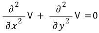
is what it is

The function V(x,y) can be expressed in an x,y,z coordinate system by representing the V(x,y) value at some x, y as the height z!

In 1D, it was possible to explain it like “the rate of change of the change is 0,” but in 2D, explaining it that way seems super hard.

When x changes by this much~~~, the rate of change of V’s change, plus when y changes by this~~~much, the rate of change of V’s change — as long as the two sum to 0 is fine,

so each of the rates of change doesn’t have to be 0 individually. That’s what I mean!!!

It’s just that that sum being 0 means, when you express V(x,y) as a surface,

“it can’t be curved!!!

That surface would have to be in a taut!!!!taut!!!! state, pulled straight ! stretched!” ☜ I agonized over this conclusion for an enormous amount of time…

If you all think it over carefully~, at some moment!! a light-bulb-flash!!! moment will come for you too.

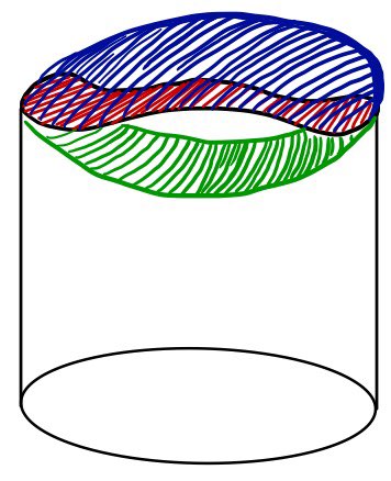
If you cut a cylinder along the black line in a wobbly wobbly way, there are infinitely many surfaces that can be defined up above there,

but among them, only the taut!taut! red surface that satisfies Laplace’s equation can be a solution???

Let’s go back to 1D for a moment lolol. It was a straight line, right? Why was it a straight line lolol. Because it was taut lolol.

Being taut in 2D — you can think of a stretched rubber sheet.

Now I’ll restate the 2 features hehe. Features of harmonic functions in 2D

1. At point (x,y), the V value equals the average of the V values at the points on a circle of radius R centered at (x,y).

2. As a result, there’s no local max or min of V. The max and min of V are always only at the boundary.

2D is doable lol, since it’s just a surface at least

Editorial clarification (2 October 2026): Two dimensions: a harmonic surface can bend.

The quoted “cannot be curved” conclusion and the identification of the red surface as the only harmonic surface are the historical author’s explanation. They are not asserted as correct here. The retained saddle example and membrane assumptions below explain the distinction.

The retained equation above is Laplace’s equation in two Cartesian coordinates.

Think of the graph as a surface whose height represents the potential. Its two second derivatives must sum to zero, but each can be nonzero. For a simple mathematical example, take

$$ V(x,y)=x^2-y^2. $$

Then

$$ V_{xx}=2,\qquad V_{yy}=-2,\qquad V_{xx}+V_{yy}=0. $$

The graph is a curved saddle. Its opposite bending in the two coordinate directions balances in the Laplacian; harmonic does not mean flat.

The sketch offers a qualitative way to imagine a fixed boundary and different surfaces spanning it. An ideal membrane with uniform tension, small slopes, and no transverse load satisfies Laplace’s equation in the linear approximation. General minimal-area surfaces instead satisfy a nonlinear equation. The drawing alone cannot establish that its red surface is exactly harmonic or minimizes area. See the UBC membrane model and Cornell’s minimal-surface equation.

For a precise averaging rule, choose a circle of radius $R>0$ centered at $(x_0,y_0)$ whose entire closed disk lies inside the harmonic region. Parameterize its circumference by

$$ \begin{aligned} x'(\theta)&=x_0+R\cos\theta,\\ y'(\theta)&=y_0+R\sin\theta. \end{aligned} $$

Writing its potential as $g(\theta)=V(x'(\theta),y'(\theta))$, the mean-value property is

$$ V(x_0,y_0)=\frac{1}{2\pi}\int_0^{2\pi}g(\theta)\,d\theta. $$

This is a uniform average around the circle, not an unweighted average of arbitrarily spaced sample points. Stanford’s mean-value theorem supplies the full harmonic-domain condition.

Three dimensions

We’ve run all the way here for the 3D Laplace equation.

But I can’t interpret it physically, I can’t.. T_T sob sob

So, following the flow from 1D and 2D, if I write down the features of harmonic functions (functions that satisfy Laplace’s equation) in 3D:

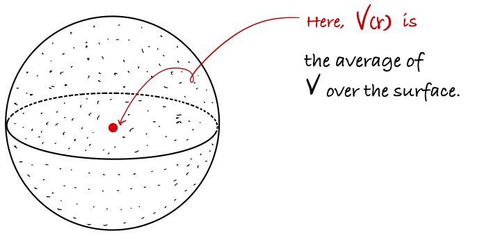
1. V(r) is the average of V over lots of spherical surfaces!!

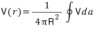
like that~

2. Same as in 1D and 2D, the min or max must be on the boundary only!

Editorial clarification (2 October 2026): Three dimensions: the average over a sphere.

The historical “lots of spherical surfaces” language refers to averages over each admissible sphere centered at the point, not an average over a collection of different spheres. The existing localized sphere label and normalization are retained.

The same idea extends to each sphere whose entire closed ball lies inside the charge-free region. In the diagram, the red dot marks the center; the black dots indicate places where the surface potential is sampled. They do not represent charges on the sphere.

Let $\mathbf r_0$ denote the center, $R>0$ the radius, and $S_R(\mathbf r_0)$ the spherical surface. Then

$$ V(\mathbf r_0)=\frac{1}{4\pi R^2}\int_{S_R(\mathbf r_0)}V(\mathbf r')\,dA'. $$

Here $dA'$ is a scalar area element. The denominator is the sphere’s area, so this is an average of potential, not electric flux. The source’s compact equation shown earlier uses the same correct normalization.

The potential can vary around the sphere; spherical symmetry is unnecessary. Each admissible radius gives the same central value. UCSB’s mean-value discussion gives the three-dimensional result.

Editorial clarification (2 October 2026): Maximum and minimum values.

The original statements exclude all interior extrema and place extrema only on the boundary. The retained correction includes the constant-function exception and the boundedness/continuity conditions.

Suppose the domain is bounded and connected, and the potential is harmonic inside and continuous on its closure. Its maximum and minimum values are attained on the boundary. A nonconstant harmonic potential has no interior local maximum or minimum. A constant solution is the exception: it attains both everywhere.

For an unbounded domain, behavior at infinity must be addressed separately, and extrema need not be attained. These qualifications belong to the maximum principle.

The saddle example helps distinguish a stationary point from an extremum: at its center the slope vanishes, but nearby values are higher in one direction and lower in another.

Boundary conditions and the next lesson

So far we’ve looked at Laplace’s equation. (We pretty much studied harmonic functions, since functions that satisfy Laplace’s equation are called harmonic functions)

But with Laplace’s equation alone, you can’t find a solution.

The value at the boundary, the very~~~ end, has to be set in order to express the inside, you know.

Well, then this question will come up: “If the values at the boundary are defined, is the V that satisfies them just that one thing???? Definitely just one????”

“The solution to that equation doesn’t necessarily have to be one, right?”

The answer to that is

“If only the boundary conditions are set, then V is, based on those boundary values, just the one!! uniquely determined.”

Is that really the case??? Prove it!! — if you say that, I’d have to tell you about the “Uniqueness theorem,”

but since it’s not super hard, I’ll skip the content explanation

See you next time with the method of images~

Editorial clarification (2 October 2026): Boundary values and uniqueness.

The author explicitly skipped the proof in the original notes. The proof and Neumann discussion below are the previously accepted editorial addition. They are not retroactively attributed to the Korean original. Complete Dirichlet data give at most one suitable solution; existence and conditions at infinity remain separate.

Laplace’s equation has many solutions by itself. Specifying the potential on the complete boundary gives a Dirichlet problem. On a bounded domain, there is at most one harmonic solution continuous to that boundary. Existence is a separate question involving the domain and boundary data. Inner boundary components also need their values; exterior problems require conditions at infinity. The electrostatic uniqueness theorem explains why complete boundary data matter.

Here is the short proof for the bounded case. Suppose two solutions have the same boundary values, and define their difference:

$$ w=V_1-V_2. $$

Linearity makes $w$ harmonic, and $w=0$ on the boundary. The maximum and minimum principles therefore give $w\leq0$ and $w\geq0$ throughout the domain. Hence $w=0$, so the two solutions coincide.

Prescribing the outward normal derivative instead gives a Neumann problem. For a bounded connected domain with a sufficiently smooth boundary, compatible data determine a solution up to an additive constant. Integrating Laplace’s equation over the domain and applying the divergence theorem requires

$$ \int_{\partial\Omega}\frac{\partial V}{\partial n}\,dA=0. $$

A reference potential fixes the remaining constant. UCSB’s treatment of Neumann data explains both compatibility and this freedom.

Uniqueness is what makes the method of images useful in the next lesson. If an image-charge construction satisfies the same field equation in the physical domain and every required boundary condition, including behavior at infinity, it gives the physical solution there. A clever construction still has to meet those conditions.

P.S. — restored from the original

P.S.

Did you know?

I have converted all the blog posts into PDFs

and am selling the PDF materials :-)

https://blog.naver.com/gdpresent/222243102313

View the original archived book photograph

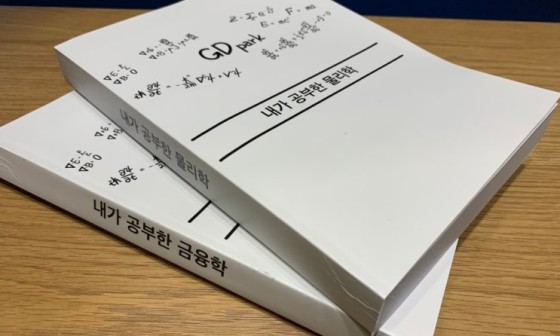
Original photograph from the archived PDF announcement: the printed books are titled Physics I Studied and Finance I Studied in Korean. The cover also carries GD park’s name and handwritten subject notes. The photograph is preserved unchanged as a record of the original printed books and is available through the link above. Photograph source: the original PDF announcement.

Blog-post PDFs (ver. 2.0) for sale (Physics I Studied, Finance I Studied)

Purchase information is below ~ Hello! If there is anything unsatisfactory in the blog posts, too much…

blog.naver.com

The sales-card excerpt is incomplete in the source. Its “too much…” ending is retained without reconstructing the missing text. The pictured covers are the original Korean printed collections; the English caption identifies their subject, without editing their photographed text.

Editorial availability note (2 October 2026). The P.S. and sales card are historical parts of the original post. A current read-only request to their destination returned Naver’s “This is a private post” notice. This article exposes no downloadable PDF attachment, and no PDF contents or present purchase availability have been verified. The original destination is retained.

Earlier editorial record — 9 September 2026

This English edition revises the original Korean post. Three image references that had pointed to unrelated diagrams were first restored from the source. Separately, the sphere annotation was translated, and three displayed formula images were replaced with typeset equations to clarify source and observation coordinates and distinguish field from potential.

Those replacements also restore the missing minus sign in the source’s field–potential relation and the missing divergence dot in its Poisson derivation. The source’s final red Poisson equation was already correct, as was its negative-Laplacian-equals-zero equation, retained above. All historical image files are preserved.

The prose corrects the derivative/jerk comparison and the claim that harmonic surfaces cannot curve. It also states the membrane approximation, the regions required for mean values, the constant-solution exception, and the conditions for boundary-value uniqueness. These are scientific corrections as well as language edits.

Original Korean notes (15 November 2014)