Polarization

I wrote this learning note on 18 November 2014. The English narrative follows the whole original sequence. Dated editorial notes distinguish source limitations and corrections; the full existing scientific edition follows as an appendix.

Original Korean learning note

Electrostatic fields inside matter

From here on, we are studying “electrostatic fields inside matter.”

Up through the previous three chapters, we did not ask, “Inside what object? Inside what material?” It was all vacuum—vacuum!

So we used epsilon-zero for the permittivity without giving it another thought.

From now on, we will ask what material we are inside.

A charge might be in vacuum, in water, or in some other material—or perhaps a gas?

The electric fields in those situations are different.

The materials respond differently to the electric field, after all!

And if the electric field differs, naturally the potential differs too.

That is the sort of thing we are going to do now.

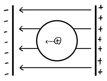
First, let us put one ordinary neutral atom in an electric field E. We want to see how the atom responds to the field.

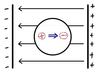
Editorial qualification — 2 October 2026. The blue arrow in source image 2 is unlabeled and points from positive toward negative charge. It must not be interpreted as the conventional electric dipole-moment vector, which points from negative toward positive charge.

Because of the electric field E, the atom’s nucleus (positive charge) shifts just a little to the left, and its electron cloud (negative charge) shifts just a little to the right!

Those displaced charges now create a new electric field inside the atom!

And if the external field E is not super-megaton strong, things will reach equilibrium.

We call this becoming “polarized.”

This polarized atom has a very small dipole moment p.

Naturally, this p will be proportional to the external electric field E.

Editorial qualification — 2 October 2026. Proportionality is a linear-response approximation. For an isotropic atom the field is the local field acting on the atom; general anisotropic response requires a polarizability tensor. These assumptions and the complete native equation are retained in the scientific appendix.

Suppose we put different kinds of atoms in that same E. Will they all have the same p? Of course not.

In the same E, some will shift a little more and others a little less.

Original source formula 3 — Induced atomic dipole moment p equals atomic polarizability alpha times the applied electric field E. The corresponding corrected native equations remain in the scientific appendix.

Writing it this way, we call alpha the “atomic polarizability.” We are looking at the atom microscopically.

For this part, it is enough to know that something like this exists.

In the classical model, we cannot really examine atoms microscopically…

Editorial qualification — 2 October 2026. Classical microscopic models can provide useful approximations. An accurate microscopic description of atoms requires quantum mechanics; the author’s informal limitation is retained as a study-note statement rather than a blanket prohibition on classical models.

(Of course, perhaps you could spend 218371273981279 hours looking at every microscopic detail. But what I mean is that doing so would miss the point.)

Up there we put an atom in an electric field; this time, let us put in a piece of dielectric made of “atoms.”

Those many atoms become polarized in the same way, so the whole piece of dielectric becomes polarized.

But now we are discussing a whole “piece” of dielectric, so let us define P.

P: dipole moment per unit volume (polarization density). This is a vector too—a vector!

For the picture we are about to consider, we pop the material into an electric field and it becomes polarized.

Then we remove the electric field again! Some materials do lose their polarization when the field is removed, but for now we will suppose it stays.

Editorial qualification — 2 October 2026. Retained polarization is an assumed configuration for this calculation. An ordinary linear dielectric generally loses its induced polarization when the applied field is removed; the example does not assert permanent polarization for every dielectric.

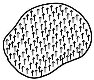
Let us suppose it has become polarized like this!

Next, let us set up the geometry like this.

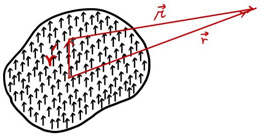
When we have a polarized material like this, with dipole moment per unit volume P,

what electric field does this polarization density produce?

What is the potential at a point r away from this object?!

The potential first!

We can just add up the potentials at r from every individual dipole.

First, the potential at r due to one dipole located at r prime is

V(r) = pr/4πε, so…

Editorial qualification — 2 October 2026. The source shorthand V(r) = pr/4πε is incomplete: it omits the vector dot product and inverse powers of separation. For a dipole at r prime the complete potential is proportional to p dotted with (r minus r prime), divided by the cube of the separation. The exact corrected native equation is preserved in the appendix.

Adding up all those potentials means the following.

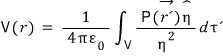
Original source formula 6 — Potential of a polarization distribution: one over four pi epsilon-zero times the volume integral of P(r prime) dotted with eta-hat, divided by eta squared. The corresponding corrected native equations remain in the scientific appendix.

Let us manipulate this expression.

Original source formula 7 — Historical gradient identity: r-hat divided by r squared is equated to gradient of one over r, with no derivative-coordinate qualifier. The corresponding corrected native equations remain in the scientific appendix.

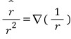
Editorial qualification — 2 October 2026. Source image 7 omits the derivative-coordinate qualifier. With the gradient taken with respect to the observation coordinate, the gradient of one over r is minus r-hat over r squared. With respect to the source coordinate, the corresponding separation identity has the opposite sign. The appendix distinguishes these derivatives explicitly.

We will use this to transform the expression a little. And since P(r prime) describes a uniformly polarized material, I will write it as P.

Editorial qualification — 2 October 2026. The subsequent general derivation must retain P(r prime), so that its divergence can describe nonuniform polarization. Uniform polarization is a special case with zero bound volume charge in the bulk; the surface charge can remain. The appendix retains the general form.

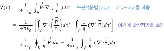
Original source formula 8 — Integration by parts followed by the divergence theorem converts the dipole integral into a surface term minus a volume-divergence term. The blue Korean annotations say to use the product rule (xy) prime equals x prime y plus x y prime, and then the divergence theorem; the right annotation is visibly clipped in the historical raster. The corresponding corrected native equations remain in the scientific appendix.

But here,

Original source formula 9 — Bound surface charge density equals P dotted with the outward normal; bound volume charge density equals minus the divergence of P. The Korean subscripts mean bound. The corresponding corrected native equations remain in the scientific appendix.

we have these relations. If we use them…!

Original source formula 10 — Potential written as a surface integral of bound surface charge over separation plus a volume integral of bound volume charge over separation, each with one over four pi epsilon-zero. The corresponding corrected native equations remain in the scientific appendix.

So when an object is polarized, inside it we have positive and negative charges: + − + − + − + −, something like that.

You can think of those charges as bound—as being held in place.

But why is that bound surface charge density the dot product of P with the normal vector perpendicular to the surface,

and why is the volume charge density inside the object the divergence of P? This part…

Editorial qualification — 2 October 2026. The source’s question omits the minus sign in the volume bound-charge relation. The source formula images and the corrected appendix give rho-b equals minus the divergence of P. The outward-normal surface relation is sigma-b equals P dotted with n-hat.

Original source formula 11 — Deliberate repeat of the bound surface and volume charge definitions from source image 9. The corresponding corrected native equations remain in the scientific appendix.

Honestly, this was very, very difficult for me too.

I came to a conclusion in my own way and carried on studying, but I think my understanding is still pretty rough.

In the next post, I will talk about those relations.

Scientific appendix: complete corrected edition

The complete scientific text and every native equation of the existing edition are retained below. Its four repeated diagram displays are references to their original occurrences above.

From here on, we are studying electrostatic fields inside matter.

In the preceding chapters, we mostly worked in vacuum, so we used the vacuum permittivity \(\varepsilon_0\) without having to discuss how a material responds. Inside water, a solid dielectric, or a gas, the charges in the material respond to an applied electric field. That response changes the resulting electric field and potential.

Let us begin with a neutral atom placed in an external electric field \(\mathbf E\).

Source image 1: Neutral atom between charged plates in a leftward external electric field

Source image 2: Polarized atom with its positive center shifted left and negative center shifted right; an unlabeled blue arrow points from positive toward negative and is not the conventional dipole-moment vector

The field shifts the positive nucleus slightly in one direction and the negative electron cloud slightly in the other. The separated charges create an internal field that opposes the displacement. Unless the applied field is so strong that the atom is ionized or driven outside the linear regime, the two effects settle into equilibrium.

The blue arrow in the retained source drawing is unlabeled and points from the positive side toward the negative side. It must not be read as \(\mathbf p\): by convention, the electric dipole moment points from negative charge toward positive charge, parallel to the applied field in this drawing.

We say that the atom has been polarized. It now carries a small induced dipole moment \(\mathbf p\). In the simplest isotropic, linear-response approximation,

\[ \mathbf p=\alpha\mathbf E_{\mathrm{loc}} \qquad\text{(isotropic, linear-response approximation)} \]

Here \(\mathbf E_{\mathrm{loc}}\) is the local field acting on the atom and \(\alpha\) is the atomic polarizability. Different atoms have different polarizabilities: the same local field produces a larger displacement in some atoms than in others. More generally, \(\alpha\) is a tensor and \(\mathbf p=\boldsymbol\alpha\cdot\mathbf E_{\mathrm{loc}}\).

For this discussion, it is enough to know what \(\alpha\) measures. A complete microscopic calculation belongs to quantum mechanics, not this classical macroscopic model. (You could spend 218371273981279 hours trying to follow every microscopic detail classically, but that would miss the point.)

From atomic dipoles to polarization density

Now replace the single atom with a piece of dielectric containing many atoms. The applied field polarizes the atoms, so the material acquires a dipole moment throughout its volume.

We describe this collectively by the polarization field

\[ \mathbf P(\mathbf r') =\frac{\text{dipole moment in a small volume around }\mathbf r'} {\text{that volume}}. \]

Thus \(\mathbf P\) is dipole moment per unit volume, and it is a vector.

Imagine that the dielectric has been polarized and that, for the moment, the polarization remains after the external field is removed. Some materials lose their polarization when the field disappears; the retained-polarization picture here is simply the configuration whose field we want to calculate.

Source image 4: Polarized dielectric filled with aligned upward dipole moments

For a uniformly polarized example, all the little dipole moments point the same way.

Source image 5: Observation geometry for a polarized dielectric, with source point r prime, observation vector r, and separation vector eta

Let \(\mathbf r'\) locate a source element inside the dielectric, let \(\mathbf r\) locate the observation point, and define

\[ \boldsymbol\eta=\mathbf r-\mathbf r', \qquad \eta=|\boldsymbol\eta|. \]

What potential does the polarized object produce at \(\mathbf r\)? We add the contributions from all its infinitesimal dipoles.

For one dipole \(\mathbf p\) at \(\mathbf r'\), the potential at \(\mathbf r\) is

\[ V_{\mathrm{dip}}(\mathbf r;\mathbf r') =\frac{1}{4\pi\varepsilon_0} \frac{\mathbf p\cdot(\mathbf r-\mathbf r')}{|\mathbf r-\mathbf r'|^3} =\frac{1}{4\pi\varepsilon_0} \frac{\mathbf p\cdot\widehat{\boldsymbol\eta}}{\eta^2}, \qquad \boldsymbol\eta\equiv\mathbf r-\mathbf r'. \]

Source correction. The original prose writes the shorthand \(V(r)=pr/(4\pi\varepsilon)\). That expression omits the vector dot product and the required inverse powers of separation. The equation above gives the complete point-dipole potential used by the following integral.

Because a source volume \(d^3r'\) carries dipole moment \(d\mathbf p=\mathbf P(\mathbf r')d^3r'\), integration gives

\[ V_{\mathrm{pol}}(\mathbf r) =\frac{1}{4\pi\varepsilon_0} \int_V \frac{\mathbf P(\mathbf r')\cdot\widehat{\boldsymbol\eta}}{\eta^2}\,d^3r', \qquad \boldsymbol\eta=\mathbf r-\mathbf r',\quad \eta=|\boldsymbol\eta|. \]

Rewriting the potential as bound-charge contributions

The sign depends on which coordinate the gradient differentiates. With \(\nabla'\) acting on the source coordinate \(\mathbf r'\), while \(\nabla\) acts on the observation coordinate \(\mathbf r\),

\[ \nabla'\!\left(\frac{1}{\eta}\right) =\frac{\boldsymbol\eta}{\eta^3} =\frac{\widehat{\boldsymbol\eta}}{\eta^2} =-\nabla\!\left(\frac{1}{\eta}\right), \qquad \boldsymbol\eta=\mathbf r-\mathbf r'. \]

Keep \(\mathbf P=\mathbf P(\mathbf r')\) for the general derivation. The product rule and divergence theorem give

\[ \begin{aligned} V_{\mathrm{pol}}(\mathbf r) &=\frac{1}{4\pi\varepsilon_0} \int_V \mathbf P(\mathbf r')\cdot\nabla'\!\left(\frac{1}{\eta}\right)\,d^3r'\\ &=\frac{1}{4\pi\varepsilon_0} \int_V\left[ \nabla'\cdot\!\left(\frac{\mathbf P(\mathbf r')}{\eta}\right) -\frac{\nabla'\cdot\mathbf P(\mathbf r')}{\eta} \right]d^3r'\\ &=\frac{1}{4\pi\varepsilon_0} \oint_{\partial V} \frac{\mathbf P(\mathbf r')\cdot\hat{\mathbf n}'}{\eta}\,da' -\frac{1}{4\pi\varepsilon_0} \int_V \frac{\nabla'\cdot\mathbf P(\mathbf r')}{\eta}\,d^3r'. \end{aligned} \]

Here \(\hat{\mathbf n}'\) is the outward unit normal on the boundary \(\partial V\) of the polarized body. Define the bound surface and volume charge densities by

\[ \sigma_b(\mathbf r')=\mathbf P(\mathbf r')\cdot\hat{\mathbf n}', \qquad \rho_b(\mathbf r')=-\nabla'\cdot\mathbf P(\mathbf r'). \]

The surface density is positive where \(\mathbf P\) points outward and negative where it points inward. The minus sign in \(\rho_b=-\nabla\cdot\mathbf P\) is essential.

The potential can therefore be written as

\[ V_{\mathrm{pol}}(\mathbf r) =\frac{1}{4\pi\varepsilon_0} \left[ \oint_{\partial V} \frac{\sigma_b(\mathbf r')}{|\mathbf r-\mathbf r'|}\,da' +\int_V \frac{\rho_b(\mathbf r')}{|\mathbf r-\mathbf r'|}\,d^3r' \right]. \]

This is the central result: a polarized object produces the same potential as a bound surface charge density \(\sigma_b\) together with a bound volume charge density \(\rho_b\).

You can picture polarization as a large collection of slightly separated positive and negative charges. In the interior, neighboring dipoles mostly cancel. A net charge can remain where \(\mathbf P\) changes through the volume or where the material ends.

If \(\mathbf P\) is uniform in the material bulk, then \(\nabla\cdot\mathbf P=0\) there and \(\rho_b=0\) in the bulk. The surface charge generally remains because \(\mathbf P\) jumps to zero outside the material, leaving \(\sigma_b=\mathbf P\cdot\hat{\mathbf n}\) on the boundary.

So why exactly do the effective charges take these forms? Here is the same definition once more, matching the original post’s deliberate recap:

\[ \sigma_b(\mathbf r')=\mathbf P(\mathbf r')\cdot\hat{\mathbf n}', \qquad \rho_b(\mathbf r')=-\nabla'\cdot\mathbf P(\mathbf r'). \]

Honestly, this part was very difficult for me when I first studied it. I formed a working picture and kept going, but it still felt rough. In the next post, I will derive these bound-charge relations more directly.