Oscillations and Damped Harmonic Motion

We’re moving at super-high speed right now… because the content is exactly~ what we learned in high school.

The only difference is that the integrals are a little~~ more complicated, so of course it feels easy, right????~~

BUT (BAM!!!!)!!!! Now it’s oscillation!!! This part is definitely going to be unfamiliar.

In high school we only did simple pendulum motion, right????? probably???

This oscillation part is super super super important, so I studied it hard!!!

Why~~ is it so important

Because in this world there are super super super many natural phenomena that can be approximated as springs!!

For example,

why hitting a wall makes a sound ☞ spring, go go

why the sky looks blue ☞ spring, go go

and the method to draw every~~~~~~~~~~~~~~~thing visible in front of our eyes is also

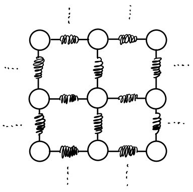
☞ spring…. hehe

These are modeling analogies: elastic vibrations and the response of bound charges can often be approximated by oscillators. Explaining blue skies also requires how light is scattered and how that scattering depends on frequency. The spring approximation is useful, but it is not a complete explanation of every phenomenon in the list.

Okay, enough intro, let’s dive in.

Why Smooth Potentials Behave Like Springs

To express the exact~ same content as the intro above a little differently,

in this world there are complicated and various potentials

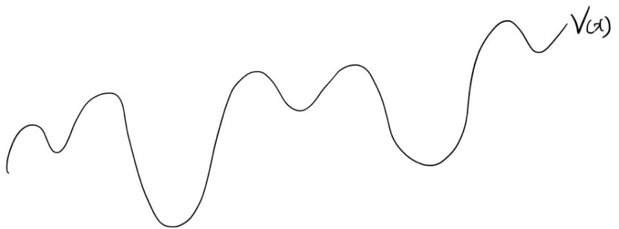
Let’s suppose there’s a potential like this. But!!! If we’re not looking at all x across the whole range

but only at the potential at some specific location~~~~~~~ then if we just do a Taylor expansion at that point,

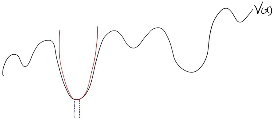
In the original 2015 notes, I wrote: “Now it’s fine to represent V(x) by the red quadratic function!!! At the x we’re interested in, the red and black functions are almoooost the same!!!!!!!” The conditions for this approximation are explained below.

Near a smooth, stable equilibrium $x_0$, the potential has a local minimum. Let $q=x-x_0$ be the displacement from that equilibrium. Taylor expansion gives

$$ \begin{aligned} V(x_0+q)={}&V(x_0)+V'(x_0)q\\ &+\frac12 V''(x_0)q^2+\cdots. \end{aligned} $$

At equilibrium $V'(x_0)=0$. If $k=V''(x_0)>0$ and the displacement is small enough that higher-order terms are negligible, the leading change in potential is $kq^2/2$: the red parabola approximates the black curve locally. That is the spring connection!!! An arbitrary point need not be an equilibrium, and a flat minimum with $V''(x_0)=0$ needs higher-order terms.

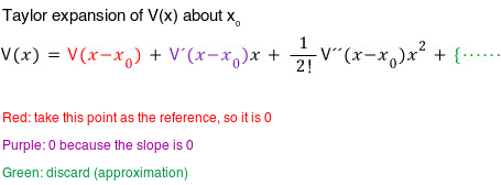
Reading the source notation: In the image above, the derivative arguments mix absolute position and displacement. Use the expansion about $x_0$ written in the text: the derivatives are evaluated at $x_0$, and their factors are powers of $q=x-x_0$. Choosing $V(x_0)=0$ fixes an arbitrary energy reference; $V'(x_0)=0$ follows from equilibrium. Dropping higher-order terms is a local approximation.

Why is it so important that the potential is quadratic in displacement….

Uh.. but… we learned something like this earlier..

In the original 2015 notes, I recalled: “We said that differentiating V(x) once with respect to x gives F(x)……????” The missing minus sign is corrected below.

The force is the negative derivative of the potential:

$$F(x)=-\frac{dV}{dx}.$$

That minus sign makes the force point downhill in potential energy.

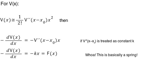
Notation correction: The retained source image mixes the equilibrium coordinate and displacement. With the definitions above, the curvature is evaluated at the fixed equilibrium, $V''(x_0)$, and the restoring force is

$$F(x_0+q)\simeq-V''(x_0)q=-kq.$$

The factor $1/2$ in the quadratic potential disappears on differentiation. In the remaining spring formulas, $x$ denotes displacement from equilibrium, so it plays the role of $q$, rather than the original absolute coordinate. We can ignore the constant $V(x_0)$ when calculating the force.

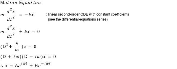
If we briefly look at the equation of motion for a spring system

Original differential equations special post

Original link-card photograph: handwritten “Differential equations special” on paper.

View the original link-card photograph

Differential equations special post.

If you’re a college STEM undergrad, you’ll encounter “(linear) differential equations” a freaking ton, so I’m going to post about this…

gdpresent.blog.me

Adding Linear Damping

Okay, now let’s step just a little closer to reality!!!!

Let’s think about resistance like friction or air resistance! That’s what I mean!!!

Based on what we learned before, let’s assume the resistive force is linear in v! (Nonlinear is super complicated;;)

Okay then, I’ll set up the equation of motion! Instead of calling the coefficient C1 like before, I’ll just call it c~~~~~

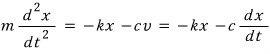
The equation of motion will be set up like this!!~~

A derivative with respect to time is marked by putting a dot above the symbol, so we call it a dot.

A derivative with respect to position is marked by placing a small stroke beside the symbol, so we call it a prime.

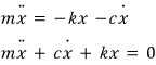
For $m>0$, $k>0$, and a viscous damping coefficient $c\geq0$, the unforced equation is

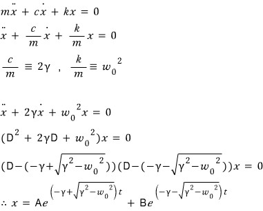
$$m\ddot x+c\dot x+kx=0.$$

This is a linear second-order differential equation with constant coefficients!! Define $\gamma=c/(2m)$ and $\omega_0=\sqrt{k/m}$. The characteristic roots are $r=-\gamma\pm\sqrt{\gamma^2-\omega_0^2}$. Distinct roots give the two-exponential solution shown below; a repeated root needs the extra factor of $t$.

For this too it’d be better to check out my differential equation special!!

But there will definitely be people who don’t want to!!!

In that case, you can check Boas Mathematical Methods Chapter 8, Section 6!!!

(To understand Section 6 well, start from Section 3 and work through it step by step!!! It’s not hard at all)

Underdamped, Critically Damped, and Overdamped Motion

<Hey, wait, wait, wait!!!!!!!

What do we do in this case!!!>

Yep, it’s simple!

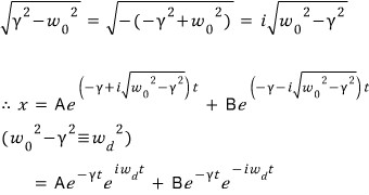
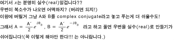
Here $x$ is clearly real, right?? What if the right-hand side turns out complex? (Just throw the imaginary part away!) Since we’re going to do that anyway, it might be easier to solve by taking $A$ and $B$ as complex conjugates! So let

$$ A=\frac{A'}{2}e^{i\theta_0}, \qquad B=\frac{A'}{2}e^{-i\theta_0}. $$

Then it is easier to make the right-hand side real! (That does not mean you absolutely have to use this particular method!!!)

Reading the source method: Here $A'$ and $\theta_0$ are real. With $\omega_d=\sqrt{\omega_0^2-\gamma^2}$, this gives

$$ \begin{aligned} x(t)&=e^{-\gamma t} \left(Ae^{i\omega_dt}+Be^{-i\omega_dt}\right)\\ &=A'e^{-\gamma t}\cos(\omega_dt+\theta_0). \end{aligned} $$

For this paired exponential expression itself to be real, its coefficients must satisfy $B=A^*$. Alternatively, take the real part of a complex solution: because this differential equation is linear with real coefficients, that real part also solves it. The amplitude-and-phase parametrization is optional; the reality condition is required.

Original Korean formula and aside

<Hey, wait, wait, wait!!!!!!!

What do we do in this case!!!>

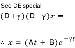
Critical-case correction: In the retained image above, the operator product $(D+\gamma)(D-\gamma)$ is a source typo. Here $D=d/dt$ and, when $\gamma=\omega_0$, the correct repeated factor is $(D+\gamma)^2$. Its solution is $(A t+B)e^{-\gamma t}$, as the image’s final line states.

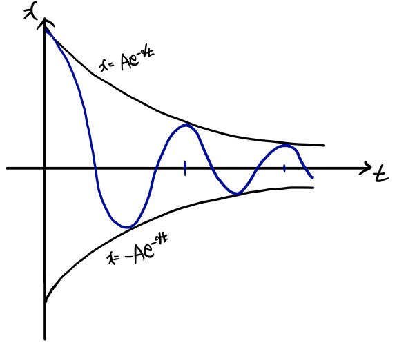
This motion is described by

This is underdamped motion, with $0<\gamma<\omega_0$ and $\omega_d=\sqrt{\omega_0^2-\gamma^2}$. A real displacement can be written

$$x(t)=e^{-\gamma t}\bigl(C\cos\omega_d t+D\sin\omega_d t\bigr).$$

The envelope decays while the object oscillates. For $c=0$, the envelope is constant and we recover undamped harmonic motion.

This kind of damped harmonic motion is something we run into all the time in everyday life, right?

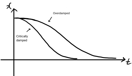Scroll sideways to read the full graph on a narrow screen.

Overdamping, $\gamma>\omega_0$, gives two distinct negative real roots:

Critical damping is

Alright! Here there’s something worth thinking about! It’s no big deal though;; hehe

Overdamped motion returns toward equilibrium without a sinusoidal oscillation. Its two exponential modes decay at different rates; the slower mode can make the return take a long time. Depending on the initial velocity, the position can still cross equilibrium once, so “nonoscillatory” does not mean every possible trajectory is monotonic. Where might damping like this be useful!??

Wouldn’t it be needed in an Equus? When you suddenly hit a bump, it goes pushuuung~ and sliiiiiiides back to the original position, so that’s what you want!!!!

Overdamping seems unconditionally good though??? Doesn’t seem like there’s any case where critical damping is needed??

Where would critical damping be needed????? In the case of a Speed Racer mega-ton supercar, rather than a pupupupushik-puuuuun shock absorber,

you’d need a shock absorber that returns to the original position in a short time!!!

Because the car needs to settle quickly, regain stability, and get back to high-speed driving, right??

The useful idea is that critical damping is the boundary between oscillatory and nonoscillatory motion. In the ideal single-mode model, for release from rest, it gives the fastest return without overshoot among critically damped and overdamped responses. Real vehicle suspensions have several coupled modes and must balance comfort, tire contact, and handling; the sedan-versus-race-car story is an intuition, not a general design rule.

hahahahahaha

Energy Loss Under Damping

Just to add a little more, let’s look at it once again from the perspective of energy.

The total mechanical energy is

$$E=\frac12mv^2+\frac12kx^2,$$

where $v=\dot x$. Differentiate both sides with respect to time $t$, and look at how $E$ changes with time:

$$ \begin{aligned} \frac{dE}{dt} &=\frac12m(2v)\dot v+\frac12k(2x)\dot x\\ &=mv\dot v+kx\dot x\\ &=m\dot x\ddot x+kx\dot x\\ &=\dot x\left(m\ddot x+kx\right)\\ &=\dot x\left(-c\dot x\right)\\ &=-c\dot x^2\leq0. \end{aligned} $$

The original source figure ends with $-c\dot x^2\ne0$. Its nonzero conclusion is qualified below.

Original Korean energy derivation

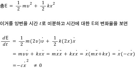
My original 2015 closing comment was: “The ‘rate of change of energy’ not being zero makes so, so, so much sense!!!!! This was damped harmonic motion with resistance!!! Common sense says the oscillation will stop eventually, so saying that E decreases isn’t wrong!!” The qualification below explains where that original wording needs care.

Qualification: The original source figure’s final “not equal to zero” is not true at every instant. The derivative is zero at a turning point where $\dot x=0$, at rest, or when $c=0$. For $c>0$, mechanical energy decreases whenever the oscillator moves; it is transferred to the surroundings. In this ideal model the motion and energy approach zero asymptotically, rather than ending at a finite time. That is exactly the energy story behind damping!!

Original post: Naver, June 19, 2015.