Vectors, Coordinate Transformations, and Polar Kinematics

Chapter 1. Vectors

We have been working with vectors again and again since high-school mathematics, so I do not think they will be particularly difficult!

The first thing about vectors that you probably learned at university, rather than in high school, was the cross product, right?

And right after learning the cross product, you were probably told, ‘You have to memorize this!’ That would be the Bac(k)-cap rule.

$$\mathbf A\times(\mathbf B\times\mathbf C)=\mathbf B(\mathbf A\cdot\mathbf C)-\mathbf C(\mathbf A\cdot\mathbf B)$$

First, what do you get from a vector triple product? Another vector!

Why? If you have learned the cross product, you should know that already…

We often memorize the expression above as a formula called the back-cap rule. But why does it take that form?

I think deriving it to understand why it works is a good thing to do.

It is simple, so please try deriving it yourselves!

Next: the coordinate-transformation matrix

The coordinate-transformation matrix was one of the basic concepts in linear algebra!

A coordinate-transformation matrix represents a linear map, or function. It is easy to analyze that map by applying it to the basis vectors of the original coordinate system!

For those concepts, please refer to ‘Linear Algebra I Studied.’ For readers who came here for classical mechanics, I will approach this as a textbook would…

First, let us express the same vector using the basis vectors of two different coordinate systems.

Then we will look for the relationship between those two coordinate systems.

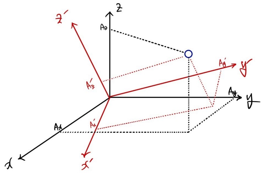
Expressing vector A in the basis of the black Oxyz coordinate system gives $\mathbf A=A_x\hat{\mathbf i}+A_y\hat{\mathbf j}+A_z\hat{\mathbf k}$ Right?

Now let us move to Ox′y′z′!

Let us find $A_{x^{\prime}}$ Taking the dot product—the projection—of vector A with the unit vector i′ along the x′ axis should give $A_{x^{\prime}}$ Shouldn’t it?

$$|A_{x^{\prime}}|=\mathbf A\cdot\hat{\mathbf i}^{\prime}=\mathbf A=(A_x\hat{\mathbf i}+A_y\hat{\mathbf j}+A_z\hat{\mathbf k})\hat{\mathbf i}^{\prime}=A_x\hat{\mathbf i}\cdot\hat{\mathbf i}^{\prime}+A_y\hat{\mathbf j}\cdot\hat{\mathbf i}^{\prime}+A_z\hat{\mathbf k}\cdot\hat{\mathbf i}^{\prime}$$

By the same principle:

$$|A_{y^{\prime}}|=A_x\hat{\mathbf i}\cdot\hat{\mathbf j}^{\prime}+A_y\hat{\mathbf j}\cdot\hat{\mathbf j}^{\prime}+A_z\hat{\mathbf k}\cdot\hat{\mathbf j}^{\prime}$$ $$|A_{z^{\prime}}|=A_x\hat{\mathbf i}\cdot\hat{\mathbf k}^{\prime}+A_y\hat{\mathbf j}\cdot\hat{\mathbf k}^{\prime}+A_z\hat{\mathbf k}\cdot\hat{\mathbf k}^{\prime}$$

Editor’s note (added): The three source projections above use absolute-value bars. A dot product with a unit basis vector gives a signed component, which can be negative. In the first line, the extra equality to the vector A and the missing dot before i′ are typographical errors. The signed-component relation is $A_{x^{\prime}}=\mathbf A\cdot\hat{\mathbf i}^{\prime}=A_x(\hat{\mathbf i}\cdot\hat{\mathbf i}^{\prime})+A_y(\hat{\mathbf j}\cdot\hat{\mathbf i}^{\prime})+A_z(\hat{\mathbf k}\cdot\hat{\mathbf i}^{\prime})$; the y′ and z′ relations follow by projecting onto j′ and k′.

Writing the three expressions above in matrix form is just a change in how we present them.

I think even a second-year high-school student could do it, because that is when we learn matrices!

So let us simply rewrite those three expressions as a matrix.

$$\begin{pmatrix}|A_{x^{\prime}}|\\|A_{y^{\prime}}|\\|A_{z^{\prime}}|\end{pmatrix}=\begin{pmatrix}ii^{\prime}&ij^{\prime}&ik^{\prime}\\ij^{\prime}&jj^{\prime}&kj^{\prime}\\ik^{\prime}&jk^{\prime}&kk^{\prime}\end{pmatrix}\begin{pmatrix}|A_x|\\|A_y|\\|A_z|\end{pmatrix}$$

Editor’s note (added): The source matrix above is retained as printed. For signed components, row a and column b of the change-of-basis matrix must be the dot product of the new basis vector a with the old basis vector b. Thus its first row is i′·i, i′·j, i′·k; the printed first-row off-diagonal entries are not consistent with the preceding projections in general. The shorthand ii′ denotes a dot product, not multiplication of vector components.

Well… very easy, right? Let me add just a little more.

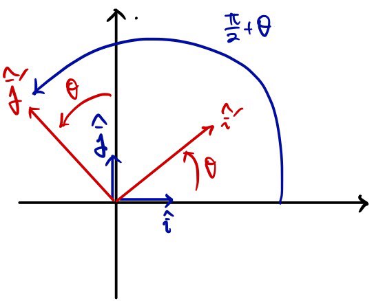
Using the same principle,

the coordinate-rotation matrix for rotating the coordinate system through theta is:

$\begin{pmatrix}\cos\theta&\sin\theta\\-\sin\theta&\cos\theta\end{pmatrix}$ You can see why this comes out this way:

$\begin{pmatrix}ii^{\prime}&ji^{\prime}\\ij^{\prime}&jj^{\prime}\end{pmatrix}$ It is because of this matrix.

It is so easy that I almost wonder whether I needed to write it down, haha.

From here it gets a little more interesting, haha—you do not learn this in high school!

Polar coordinates

Cartesian, or rectangular, coordinates just feel so natural and convenient, haha.

But sometimes using them makes things extremely complicated.

Quite often, moving away from that coordinate system makes the problem easier!

(Since I study physics, here is a physics example. In quantum mechanics, we can solve the Schrödinger equation for hydrogen. But what if we write the equation in Cartesian coordinates?

We are screwed. Not just a little screwed—you can think of it as something we simply cannot solve. But if we look at it in polar coordinates and solve it there?

Then we can solve it! Though it still is not easy, haha. Sorry about that.)

Editor’s note (added): For the three-dimensional hydrogen atom, the usual separation uses spherical polar coordinates. The equation remains physically valid in Cartesian coordinates; the issue is convenient separation and solution, not a coordinate system making the physics unsolvable.

Now we must abandon the x and y axes that we have almost believed in like a religion… sob.

Before getting started, remember that ‘coordinates’ originally meant writing the coefficients multiplying the basis vectors as an ordered pair.

Rather than saying that (2, 3) means ‘2 in x and 3 in y,’ it would be more accurate to say that we write the ordered pair (2, 3) because the vector is $2\hat{\mathbf i}+3\hat{\mathbf j}$

Using polar coordinates means changing the basis vectors.

So the coefficients are different too, and the numbers we write inside ( , ) will change, right?

Editor’s note (added): The ordered-pair description as basis coefficients applies directly to Cartesian vector components. Polar position coordinates (r, θ) are distance and angle, not the two coefficients of a position vector in the local orthonormal basis. That vector has local components (r, 0). The author’s following discussion concerns how the directions of that local basis depend on position.

First, let us get a rough idea of how the Cartesian and polar basis vectors differ.

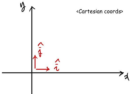
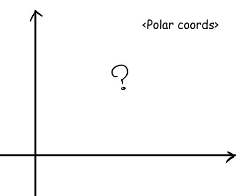
Polar coordinates do not have a fixed basis.

That means the basis keeps changing…

For those of us so used to x, y, and z coordinates, that statement may not feel intuitive.

Let us make it clear with a picture.

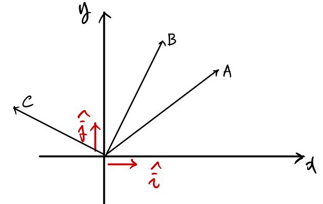
The basis vectors i and j used to describe vectors A, B, and C stay the same!

Now look at polar coordinates.

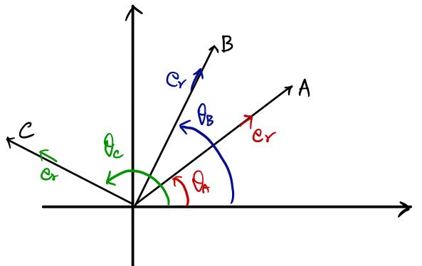
The directions of the vectors representing $\hat{\mathbf r}$ and the directions of the vectors representing $\hat{\boldsymbol\theta}$ differ from one vector to another.

In other words, the basis differs when we describe one vector and then another.

Okay.

This may seem to make things more confusing. Why did I go out of my way to explain it?

I thought that, without mentioning this, velocity and acceleration in polar coordinates might be confusing.

If you are not confused, feel free to ignore it!

Anyway, to describe velocity, acceleration, and so on in polar coordinates,

we will differentiate the position vector once with respect to time, and then take a second derivative immediately afterward.

In polar coordinates, the position vector is:

$$\mathbf r=r\hat{\mathbf r}$$

(Here r is just a number, while r-hat is the direction vector.)

Now I will differentiate it with respect to time.

$$\frac{d\mathbf r}{dt}=\frac{dr}{dt}\hat{\mathbf r}+r\frac{d\hat{\mathbf r}}{dt}$$

There we go! In Cartesian coordinates, the derivative of a basis vector was zero… But, as we saw above,

things have changed! Why? Because basis vectors are not always constant!

So now we need to work out $\frac{d\hat{\mathbf r}}{dt}$ this fellow!

The unit vector representing the direction of r would not change if it kept pointing in the same radial direction.

When that unit vector does change,

it must be because it has changed in the theta direction!

First consider the direction of the change in $\hat{\mathbf r}$ The change in the direction of r-hat can be described in the direction of $\hat{\boldsymbol\theta}$

And its amount is given by:

$$\Delta\hat{\mathbf r}=\hat{\boldsymbol\theta}\Delta\theta$$

Editor’s note (added): The displayed finite-change equality is a first-order, small-angle relation. More precisely, Δr-hat = theta-hat Δθ + O((Δθ)²); the derivative that follows is obtained in the limit Δθ → 0.

Dividing both sides by Δt,

$$\frac{d\hat{\mathbf r}}{dt}=\dot\theta\hat{\boldsymbol\theta}$$

we can explain dr/dt in this way.

Editor’s note (added): The source sentence says dr/dt, but the immediately preceding calculation is the derivative of the unit vector r-hat, not the derivative of the scalar radius r.

Along the same lines, the unit vector pointing in the $\hat{\boldsymbol\theta}$ direction changes in the $-\hat{\mathbf r}$ direction!

Why the minus sign?

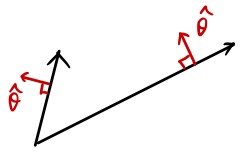
Does this give you a feel for it?

When theta changes in the positive direction, the change points in the negative radial direction!

That may still not be very intuitive, so:

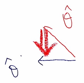
If red represents the vector before the change and blue represents it afterward,

the ‘change in the vector’ is the thick red vector, right?

That is why the vector describing the change in theta-hat points toward the center.

$$\frac{d\hat{\boldsymbol\theta}}{dt}=-\dot\theta\hat{\mathbf r}$$

Now let me write out the time derivative of the position vector in one go!

$$\mathbf v=\frac{d\mathbf r}{dt}=\frac{dr}{dt}\hat{\mathbf r}+r\frac{d\hat{\mathbf r}}{dt}=\dot r\hat{\mathbf r}+r(\dot\theta\hat{\boldsymbol\theta})$$

Done!

Let us pick up speed and move on to acceleration! Sorry for the joke.

$$\begin{aligned}\mathbf a&=\frac{d\mathbf v}{dt}=\frac{d}{dt}(\dot r\hat{\mathbf r}+r(\dot\theta\hat{\boldsymbol\theta}))\\&=\ddot r\hat{\mathbf r}+\dot r\frac{d\hat{\mathbf r}}{dt}+\dot r\dot\theta\hat{\boldsymbol\theta}+r\ddot\theta\hat{\boldsymbol\theta}+r\dot\theta\frac{d\hat{\boldsymbol\theta}}{dt}\\&=\ddot r\hat{\mathbf r}+\dot r(\dot\theta\hat{\boldsymbol\theta})+\dot r\dot\theta\hat{\boldsymbol\theta}+r\ddot\theta\hat{\boldsymbol\theta}+r\dot\theta(-\dot\theta\hat{\mathbf r})\\&=(\ddot r-r\dot\theta^2)\hat{\mathbf r}+(2\dot r\dot\theta+r\ddot\theta)\hat{\boldsymbol\theta}\end{aligned}$$

Please do not just memorize this as a formula!

All you need to do is derive it—it is simple.

So now we understand polar coordinates,

but earlier we were learning about coordinate transformations, weren’t we?

You might ask, ‘Then shouldn’t you also teach us the matrix that transforms Cartesian coordinates into polar coordinates?’

That is a question you could ask.

The mechanics textbook does not introduce it, but you can work it out very easily using a Jacobian!

Editor’s note (added): A Cartesian-to-polar coordinate map is nonlinear. Its Jacobian describes the local transformation of differentials; it is not a single constant matrix that globally converts Cartesian position coordinates to polar coordinates.

Try searching for ‘Jacobian’! Haha.

There are probably plenty of good articles elsewhere, but if you ask, I will get right to writing one!

Bye for now!

Original source and editorial provenance

Original Korean study note, June 18, 2015. The original conversational claims and invitations above are translated from the author; paragraphs explicitly labeled Editor’s note are additions. Formula screenshots are transcribed into accessible native mathematics at their original occurrences. The eight diagrams use existing, byte-preserved assets, including the two previously approved English coordinate headings.