Work-Energy Theorem and Conservative Forces

At first I welcomed this topic thinking it’d be easy. Then I read just a li~~ttle farther and realized it wasn’t going to be that simple, so I shouted, “Bye.”

What’s there in Newtonian mechanics that goes beyond the high-school level????

First of all, do they teach the chain rule in high school?????????????????????

(Sigh… am I getting old… why can’t I remember my student days?)

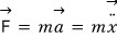
Let’s look at one-dimensional motion and keep the mass constant. Using the chain rule, we can rewrite the acceleration like this:

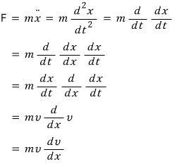
I changed an equation involving time into one involving position $x$!

I sneakily~~~ hid the time variable.

If I strip the time dependence away even more blatantly, I get

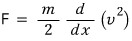
This relation is useful when we want information about position rather than time!!!!!

Now, one more thing!!!

Because the mass is constant,

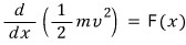
The quantity

$$ K \equiv \frac12 mv^2 $$

is called kinetic energy. It is one form of energy, rather than the definition of all energy.

Put it as a question: “How much has the energy changed as the position changes???? Was some put in, or was some taken away?” Can we put it that way?

Multiplying the differential relation $dK/dx=F$ by $dx$ and integrating gives

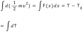
In one dimension, therefore,

$$ \Delta K=\int_{x_0}^{x}F(x')\,dx'. $$

In several dimensions the corresponding statement is

$$ \Delta K=W_{\mathrm{net}}=\int_C \mathbf F_{\mathrm{net}}\cdot d\mathbf r. $$

So work is force dotted with a differential displacement, summed along the path. It is not force “per distance.” Heh heh heh—this integral is exactly what we were taught to call work! This is the work-energy theorem!!!

Don’t be shocked when you hear this!!!! I was a little shocked.

Now suppose a force can be written in terms of a potential-energy function $V$:

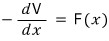
In one dimension, let’s define $V(x)$ by

$$ F(x)=-\frac{dV}{dx}. $$

Then integrating the force gives

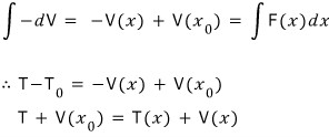
or, more cleanly,

$$ K(x)+V(x)=K(x_0)+V(x_0). $$

Super super easy stuff, right?!! This is the mechanical-energy equation for motion under that conservative force.

There is one thing we need to note:

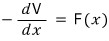
we got here by assuming that a single-valued $V(x)$ exists. In one dimension, any ordinary position-only force on an interval can be integrated to define such a potential. In more than one dimension, the real requirement is that the work between two points be path independent, equivalently that every closed-loop integral vanish:

$$ \oint \mathbf F\cdot d\mathbf r=0. $$

For a continuously differentiable force on a simply connected domain, this is equivalent to a zero curl. The domain condition matters; zero curl by itself is not enough on a region with holes.

Now someone might say, “Hey, are you trying to pull a fast one on me? Where in the world are these forces that depend only on position!!!?”

Forces with a potential are called conservative forces. Familiar examples include gravity, the electrostatic force, and the ideal spring force:

$$ \text{Gravity}=\frac{GMm}{\text{position}^{2}}\qquad \text{Electric force}=\frac{1}{4\pi\epsilon_{0}}\frac{Qq}{\text{position}^{2}}\qquad \text{Elastic force}=-k(\text{position}) $$

Original source formula

The image is a schematic reminder of position dependence. The full forces are vectors, so their exact formulas also include direction (and the appropriate sign), not just the displayed magnitudes.

The same examples in readable native notation are

$$ \begin{aligned} \mathbf F_g&=-G\frac{Mm}{r^2}\,\hat{\mathbf r},\\ \mathbf F_e&=\frac{1}{4\pi\varepsilon_0}\frac{Qq}{r^2}\,\hat{\mathbf r},\\ \mathbf F_s&=-k\mathbf x. \end{aligned} $$

Here $\hat{\mathbf r}$ points from the source to the test particle; the sign of $Qq$ determines the electrostatic direction.

We’ll learn more about these conservative forces later~~~

For a conservative force in a simply connected region,

$$ \nabla\times\mathbf F=0. $$

Looking at those examples, it can feel as if most forces in the world depend only on position….. But plenty do not.

For example:

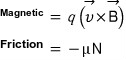
The magnetic part of the Lorentz force depends on velocity,

$$ \mathbf F_B=q\,\mathbf v\times\mathbf B, $$

but it does no instantaneous work because

$$ \mathbf F_B\cdot\mathbf v=q(\mathbf v\times\mathbf B)\cdot\mathbf v=0. $$

Kinetic friction is better written as $\mathbf F_k=-\mu_kN\,\hat{\mathbf v}$, so the minus sign and unit vector show that it opposes sliding. Velocity dependence and energy dissipation are separate questions; neither tells us that one class of force is always “more dominant” than another.

Why learn all this? One reason is that we can now study forces that do not depend only on position—air resistance, for example.

You’re riding in a car and stick your hand out the window. When is the resistive force on your hand large, and when is it small?

You’d say, “It’s large when the speed is large, and small when the speed is small~^^,” right????

Aha~ so is it proportional to speed?

Would that conclusion really be right???

Bzzzt~~~~

That observation alone doesn’t tell us whether the drag scales as speed, speed squared, or something else T_T. The answer depends on the flow regime and the object.

How would we know whether it goes with speed, speed squared, or the square root of speed? Oh… this is getting difficult… sob

In the original 2015 notes, I wrote: “Okay, okay, okay, okay—let’s imagine that the terms proportional to ‘the squares of rational numbers’ have been converted into natural-number powers by a power-series expansion.”

Scientific correction (2026-10-01): “The squares of rational numbers” is the original Korean wording. In the preceding discussion of the square root of speed, it appears to refer to fractional powers of speed; that is an inference about the intended meaning. A convergent Taylor representation requires analyticity at the expansion point. For example, $s^{1/2}$ has no Taylor series in nonnegative integer powers about $s=0$, although it has a local expansion in powers of $s-s_0$ about any $s_0>0$. Retaining only linear and quadratic drag terms is an empirical approximation for a specified range of speeds and flow conditions, not a general conversion of fractional powers into those two terms. NIST binomial expansion, NASA sphere drag.

For a simple one-dimensional model, let’s retain a linear term and a quadratic term. With positive coefficients, the signed drag force is

$$ F_{\mathrm{drag}}(v)=-c_1v-c_2|v|v. $$

The factors of $v$ make both terms oppose the motion. If we discuss only the magnitude for $v>0$, it is $c_1v+c_2v^2$, which is the convention used in the next image:

All right, then—let’s write it this way~~~!!!

The image omits the minus sign, so read its $F(v)$ as the drag magnitude. The absolute value is what lets the quadratic term be extended consistently to either direction in the signed formula above.

The coefficients $c_1$ and $c_2$ have to come from experiment for the object and fluid. For one empirical sphere model, the notes give

In the original notes I couldn’t say which scientist or engineer had done the experiments to obtain those data.

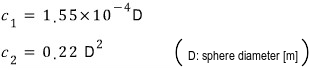
Now we can compare the magnitudes of the quadratic and linear terms:

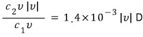
Scientific correction: The numerical coefficient in the image is incorrect. For $c_1,c_2>0$ and $v\ne0$, the values $c_1=1.55\times10^{-4}D$ and $c_2=0.22D^2$ give

$$ \begin{aligned} \frac{c_2v|v|}{c_1v} &=\frac{c_2|v|}{c_1}\\ &=\frac{0.22}{1.55\times10^{-4}}D|v|\\ &\approx 1.42\times10^3D|v|, \end{aligned} $$

with $D$ in metres and $|v|$ in metres per second for the quoted SI fit. The image shows $1.4\times10^{-3}D|v|$, which is too small by a factor of about one million.

If this dimensionless ratio is much less than 1, linear drag dominates; if it is much greater than 1, quadratic drag dominates. Hehe, let’s solve the two limiting cases.

1. Linear drag dominates

Take $v_0>0$, $x(0)=x_0$, and $F_{\mathrm{drag}}=-c_1v$.

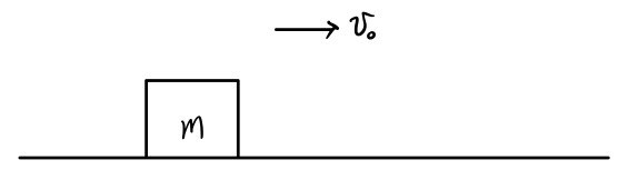
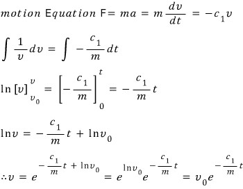
Scientific correction (2026-10-01): The source image omits the time variable in the bracketed antiderivative. The time integral is $\left[-(c_1/m)t'\right]_{t'=0}^{t'=t}=-c_1t/m$, not $\left[-c_1/m\right]_0^t$. The final exponential velocity formula in the image is correct for $v_0>0$.

The velocity is

$$ v(t)=v_0e^{-c_1t/m}. $$

Integrating once more gives

$$ x(t)-x_0=\frac{mv_0}{c_1}\left(1-e^{-c_1t/m}\right). $$

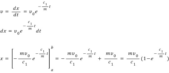
2. Quadratic drag dominates

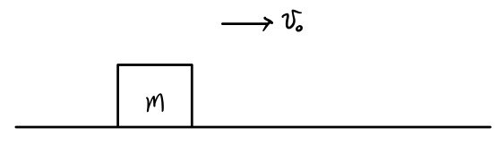
Again take $v_0>0$, so $F_{\mathrm{drag}}=-c_2v^2$ while the object continues moving to the right.

$$ \begin{aligned} &\text{Equation of motion}\quad F=ma=m\frac{dv}{dt}=-c_{2}v^{2}\\ &\int\frac{1}{v^{2}}\,dv=\int-\frac{c_{2}}{m}\,dt\\ &\left[-v^{-1}\right]_{v_{0}}^{v}=-\frac{1}{v}+\frac{1}{v_{0}}=-\frac{c_{2}}{m}t\\ &\frac{1}{v}=\frac{1}{v_{0}}+\frac{c_{2}}{m}t=\frac{m+v_{0}c_{2}t}{mv_{0}}\\ &\therefore\quad v=\frac{mv_{0}}{m+v_{0}c_{2}t}=\frac{v_{0}}{1+\frac{v_{0}c_{2}}{m}t} \end{aligned} $$

Original source formula

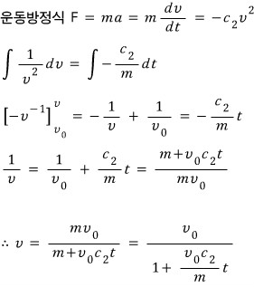
This gives

$$ v(t)=\frac{v_0}{1+(c_2v_0/m)t}. $$

Integrating the velocity should then give the displacement:

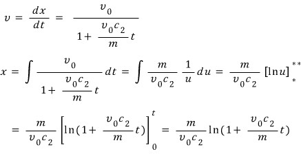
Scientific correction: The image loses a factor of $v_0$ during the substitution. If $u=1+(v_0c_2/m)t$, then $dt=m\,du/(v_0c_2)$, and the $v_0$ in the numerator cancels. Therefore the correct result is

$$ x(t)-x_0=\frac{m}{c_2}\ln\!\left(1+\frac{v_0c_2}{m}t\right), $$

not the displayed expression with prefactor $m/(v_0c_2)$. The corrected prefactor also has the required units of length.

Original post: Work-energy theorem and conservative forces (2015)